Commodity futures momentum strategy#
Create a commodity futures investment strategy based on a simple momentum signal.
Initialize SigTech
Import Python libraries:
import datetime as dtm
import numpy as np
import pandas as pd

import sigtech.framework as sig
Initialize the SigTech framework environment:
env = sig.init()
Learn more
Specify asset contract codes#
A futures contract group represents a futures strip: a series of futures contract instruments for the same underlying asset, as traded by a particular exchange.
Each futures contract group has a contract code. Create a dictionary of asset descriptions and contract codes:
assets = {
    'Corn Futures (C)': 'C ',
    'Soybean Futures (S)': 'S ',
    'Sugar Futures (SB)': 'SB',
    'Cotton Futures (CT)': 'CT',
    'Live Cattle Futures (LC)': 'LC',
    'Soybean Oil Futures (BO)': 'BO',
    'Gas Oil Futures (QS)': 'QS',
    'Heating Oil Futures (HO)': 'HO',
}
See the commodity futures section of the SigTech data browser to find commodity futures contracts and their corresponding contract codes.
Define strategy start and end dates#
Define the strategy’s start and end dates:
start_date = dtm.date(2000, 1, 8)
end_date = dtm.date(2020, 12, 8)
Create rolling future strategy objects#
Futures contracts for the same underlying asset have sequential expiry dates. When trading futures contracts, you maintain an exposure to an underlying asset by rolling from one contract to the next as each contract expires.
In the SigTech platform, you can use the sig.RollingFutureStrategy class to do this.
Learn more: Rolling Future Strategy
Define a function, create_rfs, that creates rolling future strategy objects.
def create_rfs(contract_code, start_date, end_date):
    result = None
    try:
        result = sig.RollingFutureStrategy(
            contract_code=contract_code,
            contract_sector='COMDTY',
            currency='USD',
            rolling_rule='F_0',
            start_date=start_date,
            end_date=end_date,
        ).name
    except:
        pass
    return result
In the code block above, the create_rfs function creates a rolling future strategy and returns its object name. Note that, when creating the sig.RollingFutureStrategy object:
The
rolling_ruleis set to"F_O", which specifies that the strategy should roll to the adjusted front contract. See the page on rolling future strategies for more information.The
contract_sectoris set to"COMDTY", which, along with thecontract_code, forms part of the futures contract group name. See the commodity futures section of the SigTech data browser for more.
Create a rolling future strategy object for each contract code in the assets dictionary:
rfs_strats = {
    asset: create_rfs(contract_code, start_date, end_date)
    for asset, contract_code in assets.items()
}
rfs_strats
Create trade decision signals#
A momentum strategy evaluates an asset’s performance over a given time period. It buys the asset if its price has increased, and sells the asset if its price has decreased.
Use the rolling future strategies listed in the rf_strats object to create a trade decision signal for each asset. The signal is positive (1) when the momentum strategy should buy the asset, and negative (-1) when the momentum strategy should sell the asset.
To do this, define a function, create_momentum_signals_df. The function accepts two parameters:
* `rfs_names`: A list of rolling future strategy object names.
* `window_in_days`: The time period over which to evaluate each rolling future strategy's performance.
The create_momentum_signals_df function returns a pandas DataFrame containing a momentum signal for each asset.
def create_momentum_signals_df(rfs_names, window_in_days=63):
    frames = []
    for rfs_name in rfs_names:
        rfs = sig.obj.get(rfs_name)
        pct_change_history = rfs.history().pct_change()
        rolling_mean = pct_change_history.rolling(window_in_days).mean()
        signal = np.sign(rolling_mean)
        frames.append(signal.to_frame(rfs_name))
    momentum_signals_df = pd.concat(frames, axis=1).dropna()
    return momentum_signals_df
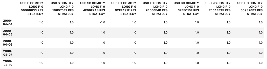
Call the create_momentum_signals_df function to create the momentum signals data frame:
momentum_signals_df = create_momentum_signals_df(rfs_strats.values())
momentum_signals_df.head()
Create the commodity momentum strategy#
Create a commodity momentum strategy from the signal data.
First, use the SigTech signal library to convert momentum_signals_df to a signal object:
signal_obj = sig.signal_library.from_ts(momentum_signals_df)
signal_obj
Next, use the sig.SignalStrategy class to create your commodity momentum strategy.
commodity_momentum_strat = sig.SignalStrategy(
    start_date=start_date,
    end_date=end_date,
    currency='USD',
    signal_name=signal_obj.name,
    rebalance_frequency='EOM',
    allocation_function=sig.signal_library.allocation.normalize_weights,
    ticker=f'Commodity Momentum Strategy'
)
In the code block above:
You supply signal data to the
sig.SignalStrategyconstructor by passing your signal’s object name in thesignal_nameparameter.To make trade decisions, the strategy examines each asset’s signal on the decision dates specified by the
rebalance_frequencyparameter.If the asset’s signal data contains a positive value on a decision date, the strategy buys the asset.
If the asset’s signal data contains a negative value on a decision date, the strategy sells the asset.
The
allocation_functionparameter specfies how the strategy allocates long and short positions. In this case, the allocation function is the signal library functionnormalize_weights, which balances the strategy to hold equal numbers of long and short positions on each decision date.
View the commodity momentum strategy’s history data:
commodity_momentum_strat.history()
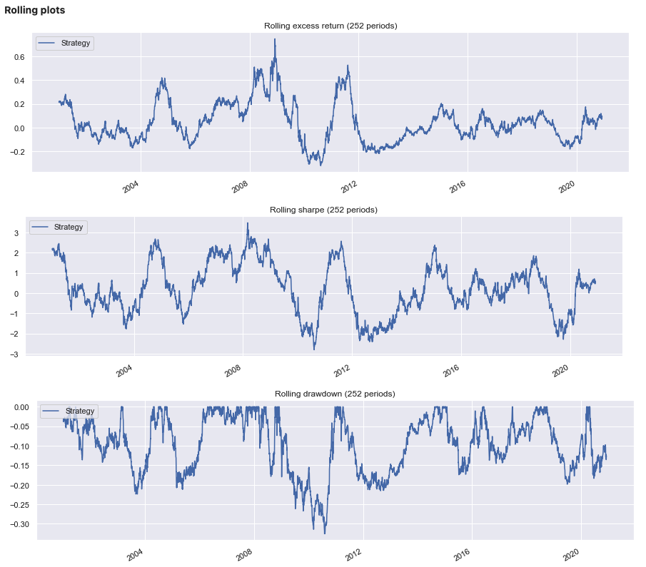
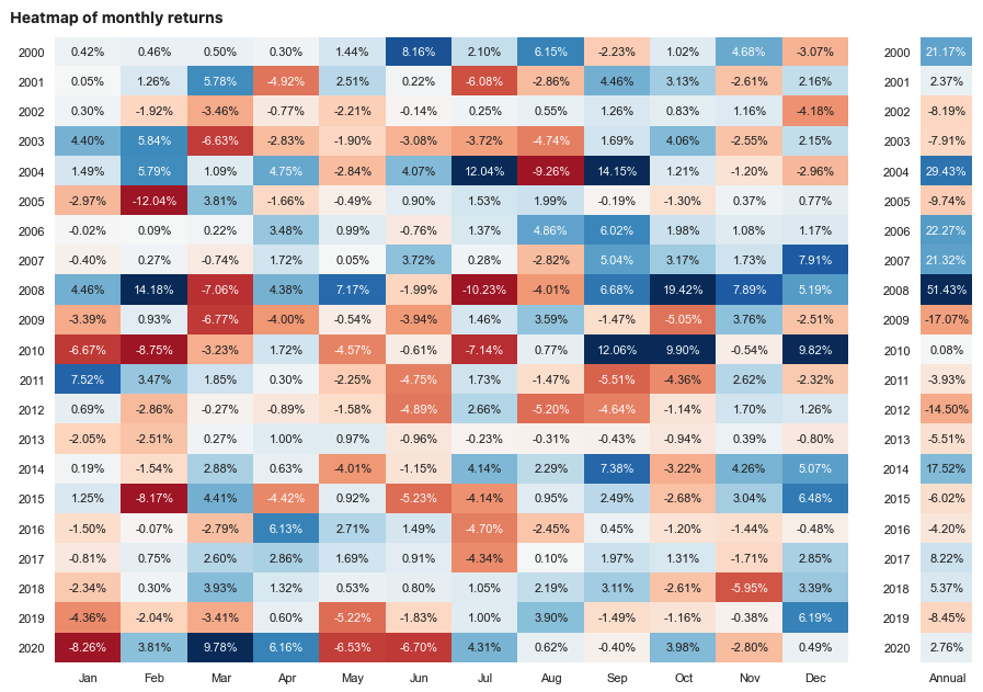
Create a performance report#
Create a performance report to show metrics, rolling performance charts, and a performance calendar.
Learn more: Performance Analytics
sig.PerformanceReport(commodity_momentum_strat).report()
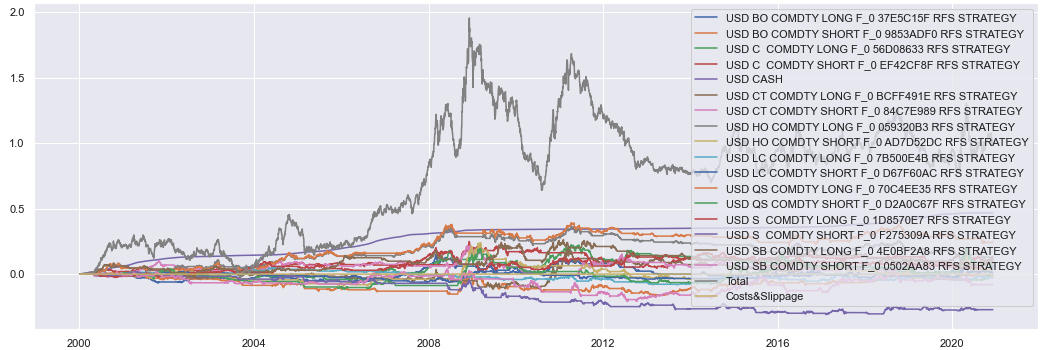
You can also analyze how each asset contributed to the overall performance of the strategy:
pnl, weight = commodity_momentum_strat.analytics.pnl_breakdown(levels=1)
pnl.plot();
Change the levels parameter of the pnl_breakdown method to investigate a layered breakdown of the strategy’s performance attribution.