Factor exposures#

The FactorExposures class enables you to create an exposure object to which different factor time series data can be attached.

To give some examples of how this object can then be used:

View a detailed report on a strategy’s exposures to given factors on a given date and through time.
Create a replicating basket for a given strategy with a defined replicating universe, by mimicking factor exposure.
Enable factor exposure to be constrained in optimisation problems.
Create Equity Factor Basket building blocks: a strategy driven by factor data.

This page details case 1 above. Cases 2 & 3 are detailed in the FactorOptimisation page, whilst 4 is explained in the EquityFactorBasket show.

Learn more: to fully understand the content of this page, see Reinvestment Strategies.

Environment#

Setting up your environment takes three steps:

Import the relevant internal and external libraries
Configure the environment parameters
Initialise the environment

from uuid import uuid4
import datetime as dtm
import numpy as np
import pandas as pd

import sigtech.framework as sig
from sigtech.framework.instruments.indices import AnalystIndex

env = sig.init()

Learn more: Setting up the environment

Class overview#

The FactorExposures class can be used with all asset classes. Equities are probably the most common use case. The FactorExposures class implements estimation methods for exposures to factors for a selection of instruments, such as performing a series of multivariate time series regressions based on a configuration.

The configuration is created by adding steps to the object:

A fit() method executes the steps on the data provided, calculating the factor loadings across the instruments.
A report() method is available to generate a report summarising the results.

Example#

This short example will showcase how to apply the FactorExposure to a number of ReinvetmentStrategy objects.

Build stock reinvestment strategies#

tickers = ['AAPL', 'AMZN', 'MSFT', 'NFLX']

Input:

tickers = ['AAPL', 'AMZN', 'MSFT', 'NFLX']
sm = env.sig_master().filter_primary_fungible().filter_primary_tradable().filter_to_last_pit_record()
ticker_mapping = sm.filter('US', 'EXCHANGE_COUNTRY_ISO2').filter_exchange_tickers(tickers).to_single_stock()
ticker_mapping = {ticker.split('.')[0]: single_stock.name
                  for ticker, single_stock in ticker_mapping.items()}
ticker_mapping

Output:

{'MSFT': 1001489.SINGLE_STOCK.TRADABLE <class 'sigtech.framework.instruments.equities.SingleStock'>[140604326065744],
 'AMZN': 1001962.SINGLE_STOCK.TRADABLE <class 'sigtech.framework.instruments.equities.SingleStock'>[140604323354960],
 'NFLX': 1025677.SINGLE_STOCK.TRADABLE <class 'sigtech.framework.instruments.equities.SingleStock'>[140615196136848],
 'AAPL': 1000045.SINGLE_STOCK.TRADABLE <class 'sigtech.framework.instruments.equities.SingleStock'>[140604323394064]

Input:

all_rs = [sig.get_single_stock_strategy(sig.obj.get(single_stock).name) for single_stock in ticker_mapping.values()]

Output:

(pid=16032) # Getting reinvestment strategy for 1001489.SINGLE_STOCK.TRADABLE
(pid=16036) # Getting reinvestment strategy for 1000045.SINGLE_STOCK.TRADABLE
(pid=16062) # Getting reinvestment strategy for 1025677.SINGLE_STOCK.TRADABLE
(pid=16037) # Getting reinvestment strategy for 1001962.SINGLE_STOCK.TRADABLE

Input:

rs_mapping = {rs.underlyer_object.exchange_ticker: rs for rs in all_rs}
rs_mapping

Output:

{'MSFT': 1001489.SINGLE_STOCK.TRADABLE REINVSTRAT STRATEGY <class 'sigtech.framework.strategies.reinvestment_strategy.ReinvestmentStrategy'>[140617254363984],
 'AMZN': 1001962.SINGLE_STOCK.TRADABLE REINVSTRAT STRATEGY <class 'sigtech.framework.strategies.reinvestment_strategy.ReinvestmentStrategy'>[140604325949520],
 'NFLX': 1025677.SINGLE_STOCK.TRADABLE REINVSTRAT STRATEGY <class 'sigtech.framework.strategies.reinvestment_strategy.ReinvestmentStrategy'>[140604323550160],
 'AAPL': 1000045.SINGLE_STOCK.TRADABLE REINVSTRAT STRATEGY <class 'sigtech.framework.strategies.reinvestment_strategy.ReinvestmentStrategy'>[140604325952400]}

Fetch factor data within the platform#

A subset of what is available:

Input:

AnalystIndex.get_names()[:5]

Output:

['US 10_INDUSTRY_PORTFOLIOS_EQ FAMA-FRENCH INDEX',
 'US 10_INDUSTRY_PORTFOLIOS_VAL FAMA-FRENCH INDEX',
 'US 12_INDUSTRY_PORTFOLIOS_EQ FAMA-FRENCH INDEX',
 'US 12_INDUSTRY_PORTFOLIOS_VAL FAMA-FRENCH INDEX',
 'US 3F_DAILY FAMA-FRENCH INDEX']

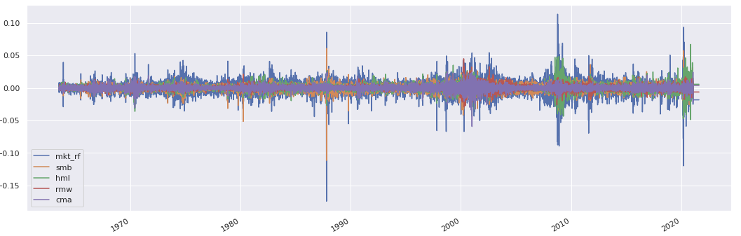
factor_data = sig.obj.get('US 5F_2X3_DAILY FAMA-FRENCH INDEX')
factor_ts = pd.concat({
    factor: factor_data.history(field=factor)
    for factor in factor_data.history_fields if factor not in ['rf']
}, axis=1) / 100
factor_ts.plot();

Compute exposures & residuals#

Create exposures object and fit regression factors:

factor_exposures = sig.FactorExposures()
factor_exposures.add_regression_factors(factor_ts)

Compute security returns and fit regression:

\[R(t) = \sum_{i} \beta_i R_i(t) + \varepsilon(t)\]

where:

the exposure to factor is, by default, the OLS estimate \(\beta_i\)
the residual at time \(t\) is \(\varepsilon(t)\)
\(R(t)\) denotes the return of the strategy at time \(t\)
\(R_i(t)\) denotes the return of factor \(i\) at time \(t\)

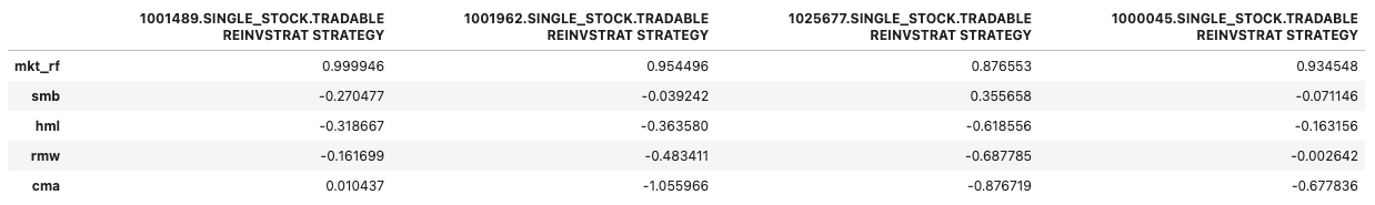
rs_returns = {rs.name: rs.history().pct_change().dropna() for rs in all_rs}
exposures, residuals = factor_exposures.fit(rs_returns)
exposures

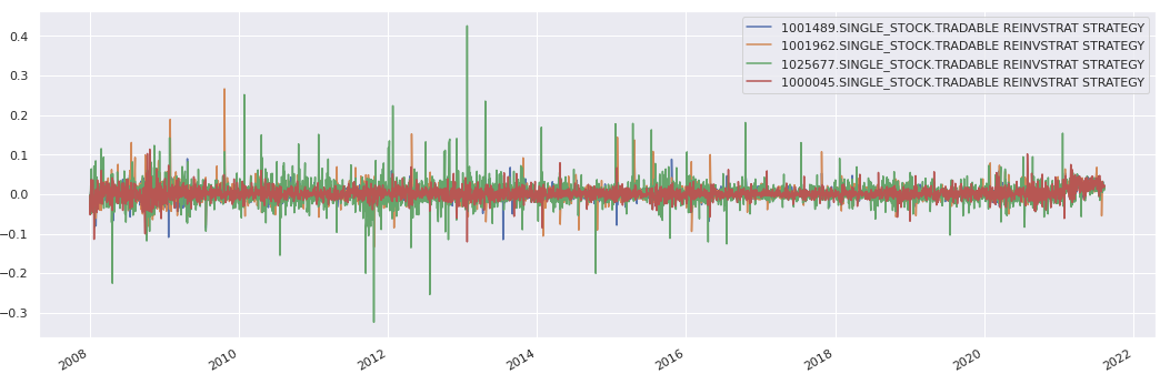
residuals.head()

residuals.plot();

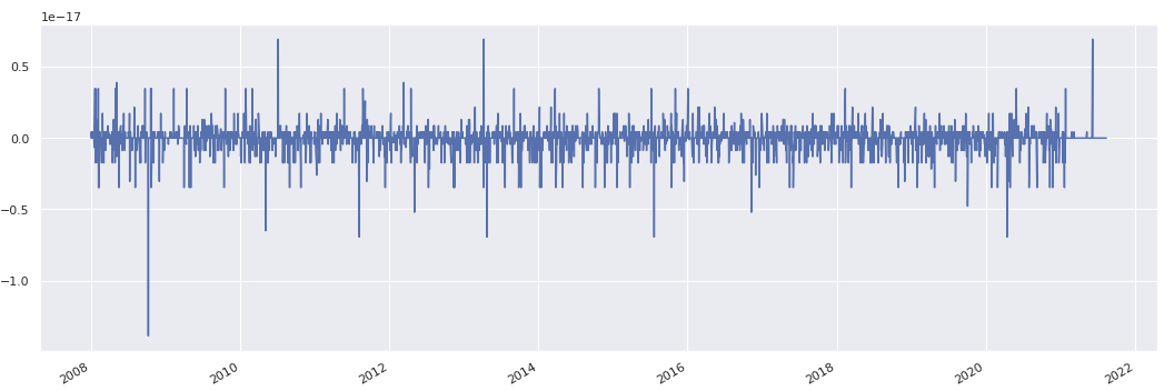
Recompute residuals manually for one strategy and compare to output:

rs = exposures.columns[0]
rs_exposures = exposures[rs]
r = rs.history().pct_change().dropna()
model_returns = (rs_exposures * factor_ts).sum(axis=1)
residuals_estimate = r - model_returns[r.index]

# numpy array
data = residuals_estimate.values - residuals[rs].values

# creating series
s = pd.Series(data, index = residuals_estimate.index)

s.plot()

Add factor data#

There are a range of methods that can be used to add factor data to a FactorExposures object:

Note: it is not necessary to be familiar with each method before the FactorExposures object is utilised.

add_regression_factors
add_cross_score

For use with EquityFactorBasket and detailed in the EquityFactorBasket page:

add_factor_exposures
add_factor_exposure_method
add_raw_factor_timeseries

add_regression_factors#

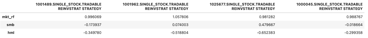
Add existing regression factor returns data as seen in the above example using the Fama-French 5-factor model:

# use 3-factor model here
factor_data = sig.obj.get('US 3F_DAILY FAMA-FRENCH INDEX')
factor_ts = pd.concat({
    factor: factor_data.history(field=factor)
    for factor in factor_data.history_fields if factor not in ['rf']
}, axis=1) / 100

factor_exposures = sig.FactorExposures()
factor_exposures.add_regression_factors(factor_ts)

Input:

factor_exposures.factor_list

Output:

['mkt_rf', 'smb', 'hml']

pd.DataFrame(factor_exposures.timeseries_factors).head()

e1, _ = factor_exposures.fit(rs_returns)
e1

add_cross_score#

View exposure to factor on ranked percentile level:

factor_exposures = sig.FactorExposures()
factor_exposures.add_regression_factors(factor_ts)

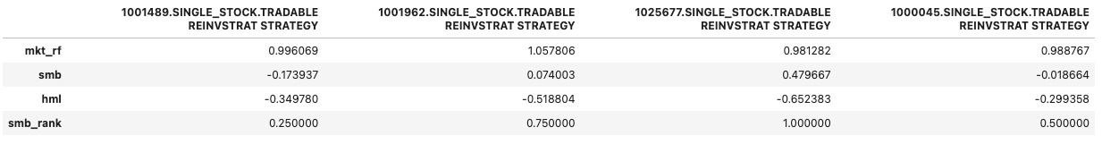
# add a cross_score for the `smb` factor called `smb_rank`
factor_exposures.add_cross_score('smb_rank', 'smb')

The updated exposures now contain the row smb_rank, indicating the percentile score for each assets exposure to the smb factor. For example, the reinvestment strategy 1001489.SINGLE_STOCK.TRADABLE REINVSTRAT STRATEGY has an smb_rank score of 0.25 since it had the lowest exposure to the smb factor out of the four assets in the universe.

e2, _ = factor_exposures.fit(rs_returns)
e2

Fit regressions#

As seen above, after regression factors have been added to the FactorExposure object, it is possible to fit a regression from a dictionary of input returns onto those factors.

More granular control over the fitting process can be gained by adding individual steps to the fitting configuration.

Input:

factor_exposures.fit_configuration

Output:

[(Index(['mkt_rf', 'smb', 'hml'], dtype='object'), {})]

factor_exposures = sig.FactorExposures()
params_dict = {
    'l1': 0.5,  # default: 0
    'l2': 0.25,  # default: 0
    'include_constant': False,  # default: True
    'normalize_if_regularized': True  # default: True
}
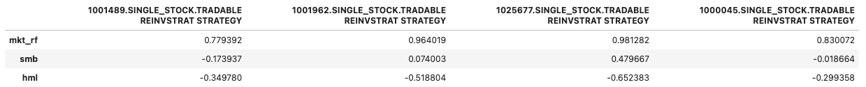
factor_exposures.add_step(factor_ts.columns, params_dict=params_dict)
factor_exposures.add_regression_factors(factor_ts)

Input:

factor_exposures.fit_configuration

Output:

[(Index(['mkt_rf', 'smb', 'hml'], dtype='object'),
  {'l1': 0.5,
   'l2': 0.25,
   'include_constant': False,
   'normalize_if_regularized': True}),
 (Index(['mkt_rf', 'smb', 'hml'], dtype='object'), {})]

e, res = factor_exposures.fit(rs_returns)
e

Possible to clear configuration:

Input:

factor_exposures.clear_steps()
factor_exposures.fit_configuration

Output:

[]

Reporting#

Fit exposures again:

factor_exposures = sig.FactorExposures()
factor_exposures.add_regression_factors(factor_ts)
e, r = factor_exposures.fit(rs_returns)

Rolling exposures#

Create example portfolios:

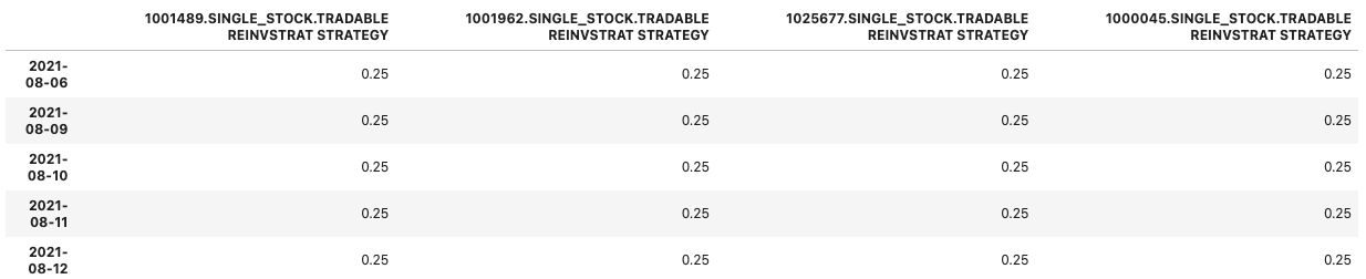
rs_histories = pd.concat({rs.name: rs.history() for rs in all_rs}, axis=1).dropna()

ew_portfolio = 1 / len(all_rs) + 0 * rs_histories
ew_portfolio.tail()

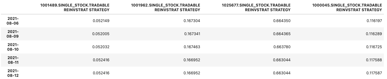
perf_weighted_portfolio = rs_histories.divide(rs_histories.sum(axis=1), axis=0)
perf_weighted_portfolio.tail()

Compute exposure of portfolios to factors through time:

ew_exp = factor_exposures.rolling_exposures(ew_portfolio)
perf_exp = factor_exposures.rolling_exposures(perf_weighted_portfolio)
ew_exp.columns = [f'ew_{c}' for c in ew_exp]
perf_exp.columns = [f'perf_{c}' for c in perf_exp]
df = pd.concat([ew_exp, perf_exp], axis=1)

(len(all_rs) * df).tail()

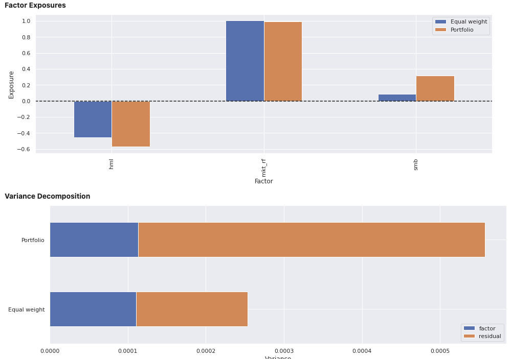
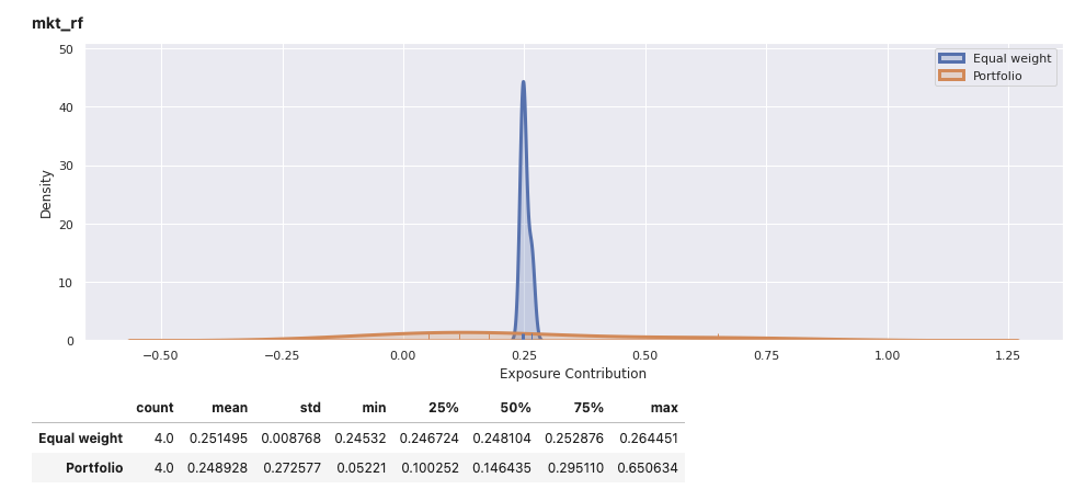
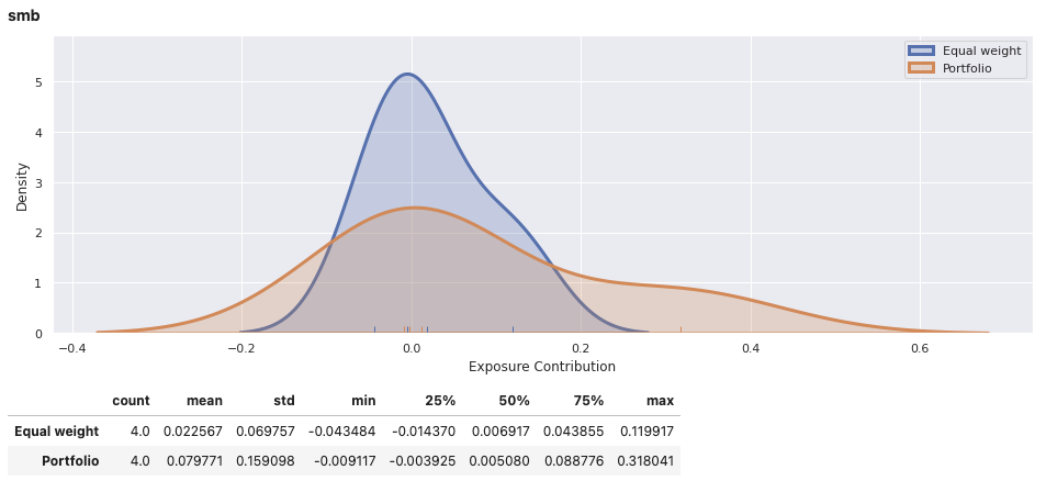
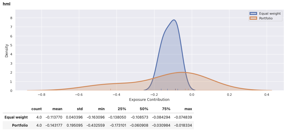
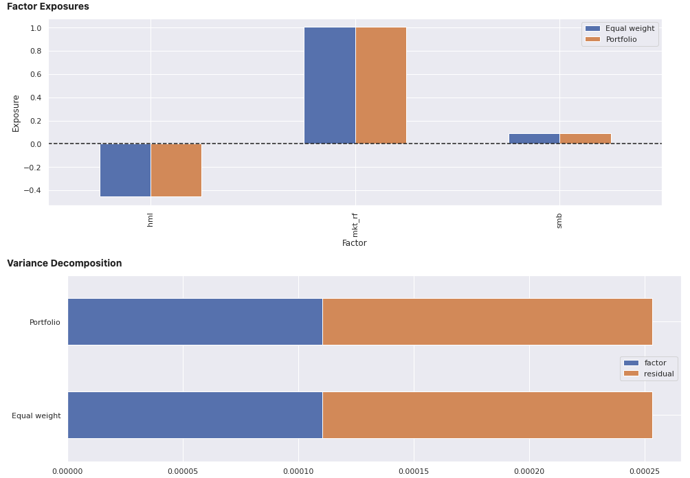
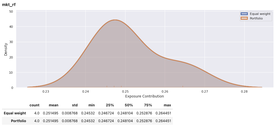
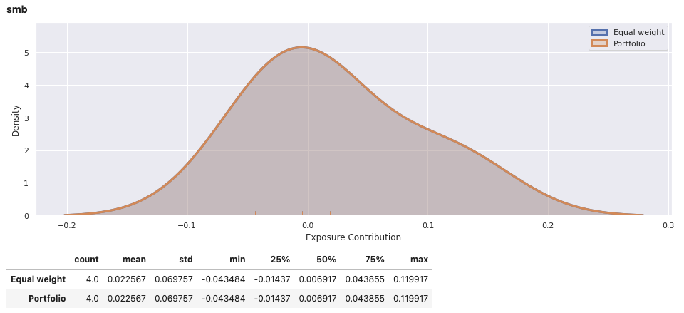
Fixed portfolio report#

View the report for an individual portfolio, including an equally weights combination of securities within the portfolio for comparison. In addition to factor exposure, there is also variance decomposition and density plots of the weighted exposures of securities within the portfolio.

factor_exposures.report(ew_portfolio.iloc[-1])

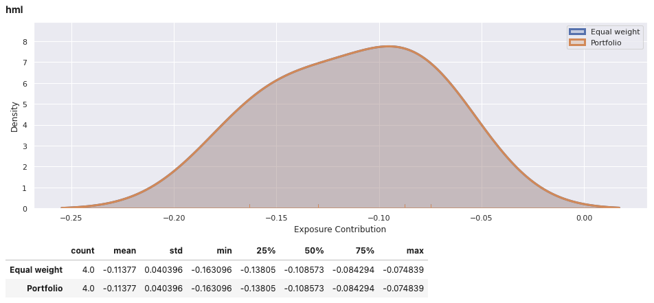
factor_exposures.report(perf_weighted_portfolio.iloc[-1])

Table of Contents

Factor exposures

Factor exposures#

Environment#

Class overview#

Example#

Build stock reinvestment strategies#

Fetch factor data within the platform#

Compute exposures & residuals#

Add factor data#

add_regression_factors#

add_cross_score#

Fit regressions#

Reporting#

Rolling exposures#

Fixed portfolio report#