Reinvestment strategy#
A reinvestment strategy creates an exposure to a single primary tradable stock instrument. In the SigTech platform, reinvestment strategies are instances of the ReinvestmentStrategy class, which can be used to handle corporate actions for underliers.
Inheriting from the DailyStrategy base class, ReinvestmentStrategy adjusts for corporate actions throughout the historical timeline of a strategy, including stock splits, takeovers, mergers, and spinoffs.
Environment#
Import Python libraries and initialize the SigTech framework environment:
import datetime as dtm
import numpy as np
import pandas as pd

import sigtech.framework as sig

env = sig.init()
Learn more: SigTech framework environment
Retrieve a primary tradable single stock object#
Define a function get_primary_tradable to:
Accept
mic, an exchange operating Market Identifier Code (MIC), andticker, a stock tickerFilter SigTech’s point-in-time stock data for matching records
Return a primary tradable single stock object
def get_primary_tradable(mic, ticker):
    return env.sig_master()\
        .filter_to_last_pit_record()\
        .filter_primary_fungible()\
        .filter_primary_tradable()\
        .filter_operating_mic(operating_mics=mic)\
        .filter_exchange_tickers(exchange_tickers=ticker)\
        .to_single_stock()[f"{ticker}.{mic}"]
Learn more: For more information on finding stock tickers and filtering SigTech’s point-in-time stock data, see Single stocks.
Use the get_primary_tradable function to retrieve the primary tradable instrument for Apple stocks in the US:
Input:
stock_obj = get_primary_tradable("XNAS", "AAPL")
stock_obj
Output:
1000045.SINGLE_STOCK.TRADABLE <class 'sigtech.framework.instruments.equities.SingleStock'>[140232241122000]
Alternatively, use the sig.obj.get utility function to retrieve the SingleStock object by its object name:
Input:
ticker = "1000045.SINGLE_STOCK.TRADABLE"
stock_obj = sig.obj.get(ticker)
stock_obj
Output:
1000045.SINGLE_STOCK.TRADABLE <class 'sigtech.framework.instruments.equities.SingleStock'>[140232241122000]
Retrieve unadjusted price data#
Retrieve a single stock object’s unadjusted price series and plot the data:
stock_obj.history(field="LastPrice").plot()
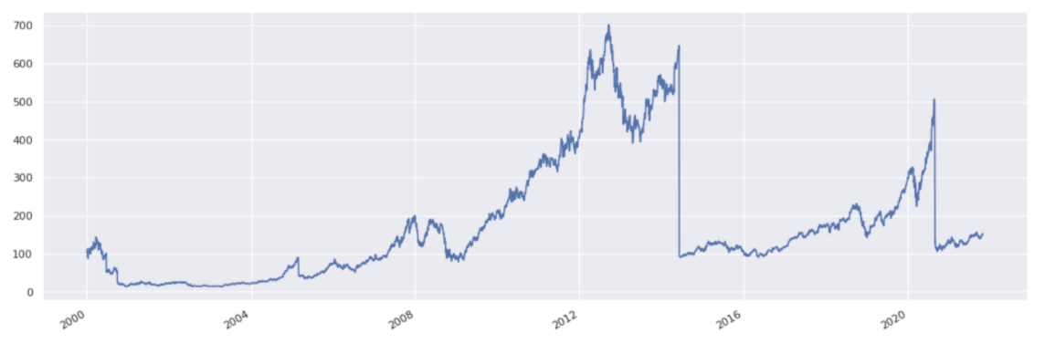
The large drops in the instrument’s price correspond to stock splits. To get more detail, examine the corporate actions for the single stock instrument:
Input:
corporate_actions = sig.internal.equities.corporate_actions.corporate_actions
splits = [
    ca for ca in stock_obj.corporate_actions()
    if isinstance(ca, corporate_actions.StockSplit)
]
splits
Output:
[StockSplit(Stock Split on 2000-06-21),
 StockSplit(Stock Split on 2005-02-28),
 StockSplit(Stock Split on 2014-06-09),
 StockSplit(Stock Split on 2020-08-31)]
Retrieve price data adjusted for corporate events#
To retrieve a single stock object’s historical price data, adjusted for specified corporate actions, use the object’s adjusted_price_history method.
The adjusted_price_history function gives the instrument’s price data when dividends are reinvested in the same instrument. You can specify how to handle special and regular dividends, and the associated tax. The method also adjusts for corporate events like stock splits, and incorporates these events into the price series.
Parameter |
Default |
Behavior |
|---|---|---|
|
None (Required) |
When |
|
None (Required) |
When |
|
|
When |
Example: AAPL#
aapl = get_primary_tradable("XNAS", "AAPL")
adjusted_data_aapl = pd.concat({
    'Unadjusted': aapl.history(),
    'AdjustedAll': aapl.adjusted_price_history(
        adjust_regular_cash=True,
        adjust_special_cash=True,
    ),
    'AdjustedRegularOnly': aapl.adjusted_price_history(
        adjust_regular_cash=True,
        adjust_special_cash=False,
    ),
    'AdjustedSpecialOnly': aapl.adjusted_price_history(
        adjust_regular_cash=False,
        adjust_special_cash=True,
    ),
    'AdjustedNoDivs': aapl.adjusted_price_history(
        adjust_regular_cash=False,
        adjust_special_cash=False,
    ),
}, axis=1)
adjusted_data_aapl /= adjusted_data_aapl.iloc[0]
adjusted_data_aapl.plot(title="AAPL Prices Series")
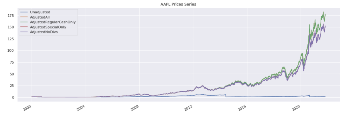
In the data above, there are stock splits and regular cash dividends, but no special cash dividends. The stock splits are accounted for in the adjusted series data.
Example: TSLA#
tsla = get_primary_tradable("XNAS", "TSLA")
adjusted_data_tsla = pd.concat({
    'Unadjusted': tsla.history(),
    'AdjustedAll': tsla.adjusted_price_history(
        adjust_regular_cash=True,
        adjust_special_cash=True,
    ),
    'AdjustedRegularOnly': tsla.adjusted_price_history(
        adjust_regular_cash=True,
        adjust_special_cash=False,
    ),
    'AdjustedSpecialOnly': tsla.adjusted_price_history(
        adjust_regular_cash=False,
        adjust_special_cash=True,
    ),
    'AdjustedNoDivs': tsla.adjusted_price_history(
        adjust_regular_cash=False,
        adjust_special_cash=False,
    ),
}, axis=1)
adjusted_data_tsla /= adjusted_data_tsla.iloc[0]
adjusted_data_tsla.plot(title="TSLA Prices Series")
As no dividends have been paid by TSLA, altering the input arguments to adjusted_price_history does not impact the resulting time series.
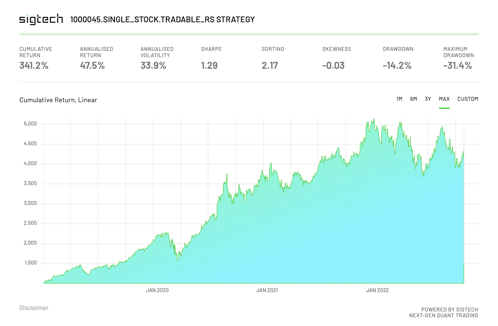
Create a reinvestment strategy#
A SigTech reinvestment strategy automatically handles corporate actions, using price data adjusted for corporate actions and reinvesting dividends, and optionally accounts for transaction costs.
The following example creates a reinvestment strategy using ReinvestmentStrategy. It takes the instrument’s string identifier/ticker AAPL_RS as an underlier parameter:
Input:
start_date = dtm.datetime(2018, 1, 1)
end_date = dtm.datetime(2024, 1, 1)
aapl_rs = sig.ReinvestmentStrategy(
    start_date=start_date,
    end_date=end_date,
    currency=aapl.currency,
    underlyer=aapl.name,
    ticker=f"AAPL_RS",
)
aapl_rs
Output:
AAPL_RS STRATEGY <class 'sigtech.framework.strategies.reinvestment_strategy.ReinvestmentStrategy'>[140049016689296]
View the reinvestment strategy’s history data:
Input:
aapl_rs.history().tail()
Output:
2023-12-22    1543.380355
2023-12-26    1538.995709
2023-12-27    1539.792914
2023-12-28    1543.220903
2023-12-29    1534.850228
Name: (LastPrice, EOD, AAPL_RS STRATEGY), dtype: float64
The strategy’s trading days are determined by its holiday calendar. Retrieve the strategy’s holiday calendar:
Input:
aapl_cal_name = aapl_rs.underlyer_object.holidays()
aapl_cal = sig.obj.get(aapl_cal_name)
aapl_cal
Output:
'NYSE(T) CALENDAR'
About the ReinvestmentStrategy class#
The sig.ReinvestmentStrategy class inherits fields and methods from the Strategy class:
Input:
issubclass(sig.ReinvestmentStrategy, sig.Strategy)
Output:
True
Like all strategies, a reinvestment strategy has access to the plotting and analytics wrappers used by sig.Strategy:
Input:
plot_wrapper = aapl_rs.plot
plot_wrapper
Output:
<sigtech.framework.strategies.components.plot_wrapper.PlotWrapper at 0x7fd24ce10fd0>
Input:
analytics_wrapper = aapl_rs.analytics
analytics_wrapper
Output:
<sigtech.framework.strategies.components.analytics_wrapper.AnalyticsWrapper at 0x7fd24cee7bd0>
plot_wrapper.performance()
A reinvestment strategy also has access to properties defined on the parent class:
print(aapl_rs.direction)
print(aapl_rs.initial_cash)
print(aapl_rs.include_trading_costs)
print(aapl_rs.total_return)
You can use Strategy parameters when you create a reinvestment strategy:
aapl_rs_2 = sig.ReinvestmentStrategy(
    start_date=start_date,
    end_date=end_date,
    currency=aapl.currency,
    underlyer=aapl.name,
    ticker=f"AAPL_RS",

    include_trading_costs=True,
)
aapl_rs_2
Strategy details and parameters#
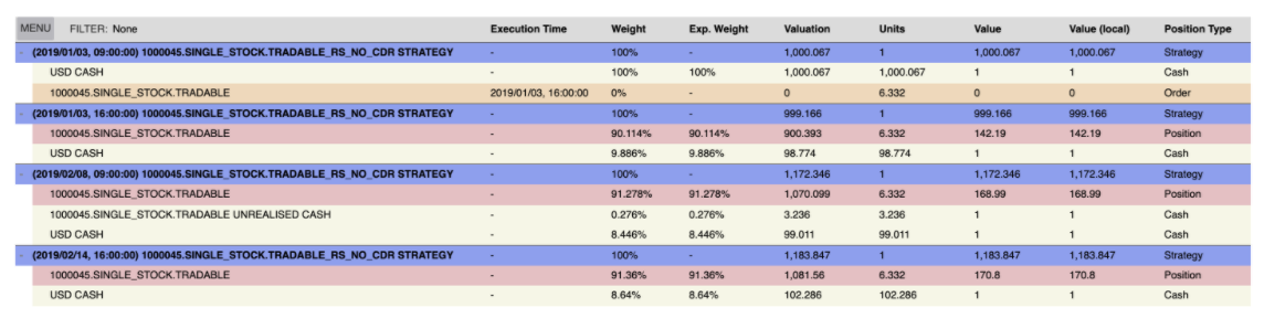
Analyzing the basic strategy at the level of TOP_POSITION_CHG_PTS:
Generation of an initial order on the underlying stock [2019/01/03, 09:00:00].
Execution of the initial order on the underlying stock [2019/01/03, 16:00:00].
Cash dividend going ex and being considered part of ‘UNREALISED CASH’ [2019/02/08, 09:00:00].
Generation of an order to reinvest dividends paid by the stock back into the stock [2019/02/14, 09:00:00].
Execution of the above order to reinvest dividend distribution [2019/02/14, 16:00:00].
To ensure that strategy action times are displayed locally, set timezone to be that of the security.
Note: The default timezone is UTC.
Input:
import pytz
local_timezone = pytz.timezone(stock_obj.exchange().timezone)
local_timezone.zone
Output:
'America/New_York'
start_date = dtm.datetime(2023, 1, 1, tzinfo=local_timezone)
aapl_rs.plot.portfolio_table(
    dts="TOP_POSITION_CHG_PTS",
    start_dt=start_date,
    end_dt=start_date + dtm.timedelta(days=60),
    tzinfo=local_timezone
)
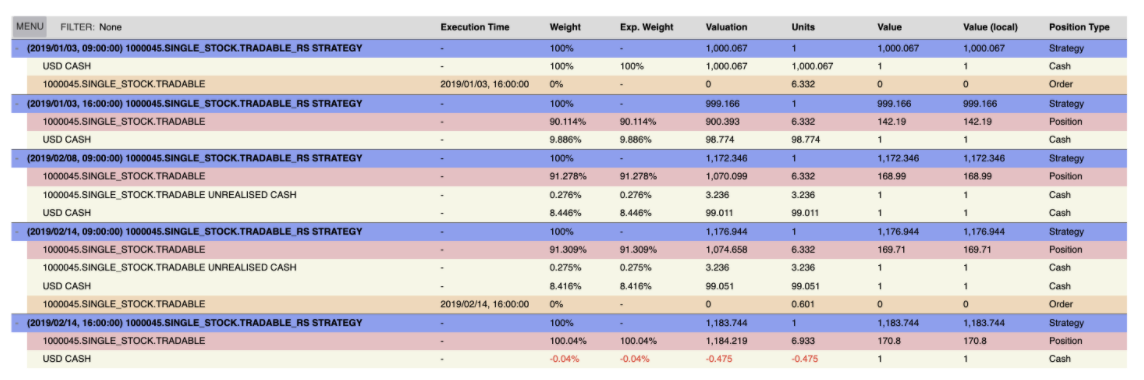
Dividends#
Continuing from the above outline, the position in 1000045.SINGLE_STOCK.TRADABLE UNREALISED CASH at [2019/02/14, 09:00:00] is dividend proceeds.
ca = aapl_rs.underlyer_object.corporate_actions()
first_dividend_effective_dtm = dtm.datetime(2019, 2, 8, 9, tzinfo=local_timezone)
dividend = [c for c in ca \
        if c.effective_date == first_dividend_effective_dtm.date()][0]
dividend

Input:
print(f"Effective Date: {dividend.effective_date}")
print(f"Payment Date: {dividend.payment_date}")
Output:
Effective Date: 2019-02-08
Payment Date: 2019-02-14
Verify dividend cash calculation:
stock_position = aapl_rs.inspect.positions_df().tz_convert(local_timezone)
stock_position.head()
Input:
units = stock_position.loc[:first_dividend_effective_dtm].iloc[-1, 0]
print(f"Stock Units: {round(units, 3)}")
Output:
Stock units: 6.332
Input:
default_wht = 0.3 # default 30% withholding tax
dividend_cash = units * dividend.dividend_amount * (1 - default_wht)
print(f"Dividend Cash: {round(dividend_cash, 3)}")
Output:
Dividend cash: 3.236
Reinvesting cash dividends#
By default, dividends received are reinvested in the underlying stock. The parameter reinvest_cash_dividends provides you with control over this logic.
rs_no_cdr = sig.ReinvestmentStrategy(
    start_date=start_date,
    end_date=end_date,
    currency=aapl.currency,
    underlyer=aapl.name,

    # specify no cash dividend reinvestment
    reinvest_cash_dividends=False,

    ticker=f"{aapl.name}_RS_NO_CDR"
)

rs_no_cdr.build()
With this change, the order to reinvest cash from the dividend on 14th February has disappeared. Instead, the unrealized cash from the dividend effective date becomes part of realized ‘USD CASH’ on the dividend payment date.
rs_no_cdr.plot.portfolio_table(
    dts="TOP_POSITION_CHG_PTS",
    start_dt=start_date,
    end_dt=start_date + dtm.timedelta(days=60),
    tzinfo=local_timezone
)
Withholding tax rates#
Withholding tax (WHT) time series can be accessed from a stock object.
Input:
stock_obj.dividend_withholding_tax_ts()
Output:
1990-01-01 0.3
Name: Dividend Withholding Tax, dtype: float64
A particular WHT rate can be set by using the withholding_tax_override parameter.
Create an RS with no WHT:
rs_no_wht = sig.ReinvestmentStrategy(
    start_date=start_date,
    end_date=end_date,
    currency=stock_obj.currency,
    underlyer=aapl.name,

    # specify no withholding tax rate
    withholding_tax_override=0.0,

    ticker=f"{aapl.name}_RS_NO_WHT"
)

rs_no_wht.build()
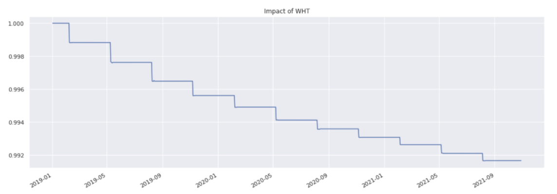
The following plot shows the ratio of the value of the RS with 30% WHT to the RHS with 0% WHT:
df = pd.concat({
    "RS_WHT": aapl_rs.history(),
    "RS_NO_WHT": rs_no_wht.history(),
}, axis=1)
df["RATIO"] = df["RS_WHT"] / df["RS_NO_WHT"]
df["RATIO"].plot(title="Impact of WHT")
rs_no_wht.plot.portfolio_table(
    dts="TOP_POSITION_CHG_PTS",
    start_dt=start_date,
    end_dt=start_date + dtm.timedelta(days=60),
    tzinfo=local_timezone
)
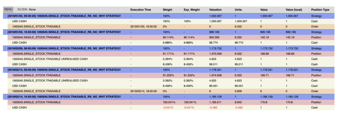
The jumps in ratio between the two versions of the RS occur on dividend effective dates.
Fetch regular cash dividends:
from sigtech.framework.internal.equities.corporate_actions.corporate_actions import RegularCashDividend
dividends = [
    c for c in ca if isinstance(c, RegularCashDividend)
    if c.payment_date >= dtm.date(2018,1,1)
]
ratio_changes = sorted(df.RATIO.pct_change().sort_values(). \
                head(len(dividends)).index.tolist())
payment_dates = [c.effective_date for c in dividends \
                if c.effective_date < dtm.date(2024,1,1)]
Tracking#
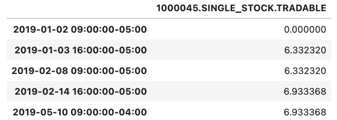
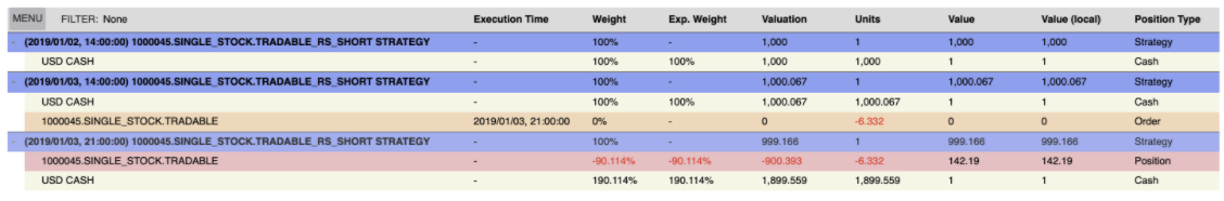
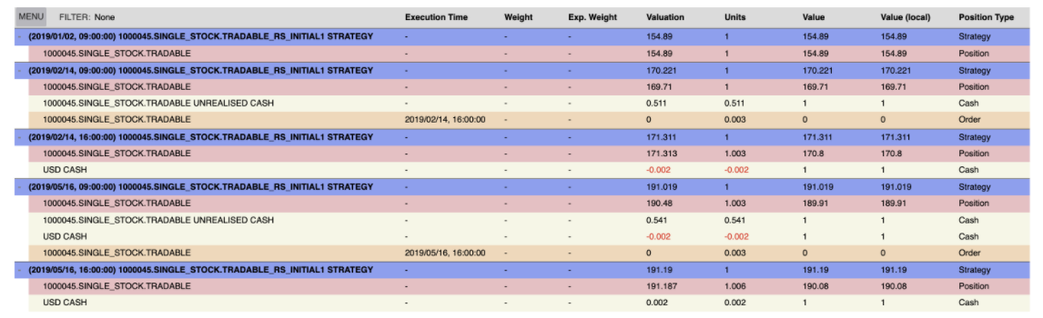
Revisiting the first Reinvestment Strategy created, the portfolio table shows that the initial position in stock is actually 90.114% [2019/01/03 16:00:00]:
aapl_rs.plot.portfolio_table(
    dts="TOP_ORDER_PTS",
    start_dt=start_date,
    end_dt=start_date + dtm.timedelta(days=1),
    tzinfo=local_timezone
)
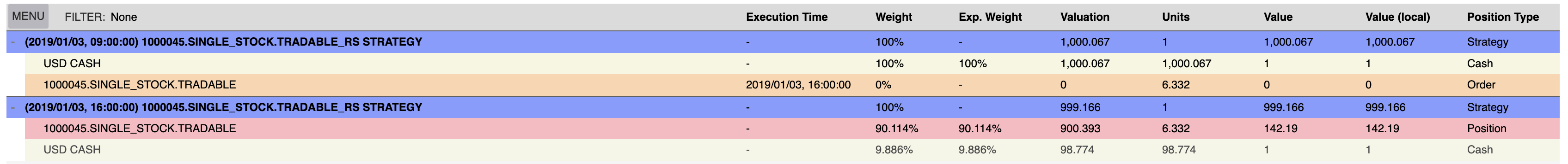
The weight of an instrument held within a strategy, assuming the instrument is in the same currency as the strategy, can be computed as: (units_held * unit_price) / strategy_price
Check this calculation directly:
Input:
value_date = pd.Timestamp(2019, 1, 3)
rs_price = aapl_rs.valuation_price(value_date)
rs_price
Output:
999.1662739994936
Input:
stock_price = stock_obj.valuation_price(value_date)
stock_price
Output:
142.19001
Input:
stock_obj.history().loc[value_date]
Output:
142.19001
Input:
value_dt = aapl_rs.valuation_dt(value_date)
stock_units = stock_position.loc[:value_dt].iloc[-1, 0]
stock_units
Output:
6.332320162107397
Agreement with the above portfolio table:
Input:
print(
f"Stock Exposure: {round(100 * (stock_price * stock_units) / rs_price, 3)}%"
)
Output:
Stock Exposure: 90.114%
The reason this exposure does not exactly match the target exposure of 100% is that the sizing, or determination of the number of shares to trade, is done using the prior day’s close. This closely resembles the experience of a trader with access to End of Day (EOD) prices.
In most cases, the difference between target weight and realised weight would not be this large. In this particular case, AAPL experienced a large negative move on the day of execution (-9.96%).
Input:
100 * stock_obj.history().pct_change().loc[value_date]
Output:
-9.960733282674761
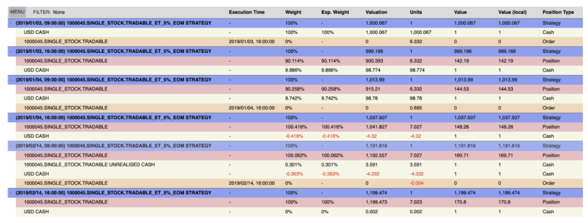
The enable_tracking parameter will cause an RS to trade toward full exposure on a schedule you provided (tracking_frequency, default SOM).
An optional tracking_threshold can also be set (default 1bp) that controls whether these tracking trades should be executed. For example, the threshold is 1%, the current exposure is 99.5%, so no action takes place.
rs_et = sig.ReinvestmentStrategy(
    start_date=start_date,
    end_date=end_date,
    currency=stock_obj.currency,
    underlyer=ticker,

    # enable tracking
    enable_tracking=True,
    tracking_frequency="EOM",
    tracking_threshold=0.05,

    ticker=f"{ticker}_ET_5%_EOM",
)
rs_et.build()
An additional trade is now scheduled on 2019/01/04.
Since this brings the exposure to within the threshold of the target, no further trades are implemented until the dividend is reinvested in February.
rs_et.plot.portfolio_table(
    dts="TOP_ORDER_PTS",
    start_dt=start_date,
    end_dt=start_date + dtm.timedelta(days=60),
    tzinfo=local_timezone
)
Setting very low thresholds and a very regular threshold_frequency can impact performance.
Input:
rs_et_1bd = sig.ReinvestmentStrategy(
    start_date=start_date,
    end_date=end_date,
    currency=stock_obj.currency,
    underlyer=ticker,
    enable_tracking=True,
    tracking_frequency="1BD",
    tracking_threshold=0.0001,
    ticker=f"{ticker}_ET_1bp_1BD",
)
%time rs_et_1bd.build()
Output:
CPU times: user 734 ms, sys: 17 µs, total: 734 ms
Wall time: 732 ms
Input:
rs_et_1m = sig.ReinvestmentStrategy(
    start_date=start_date,
    end_date=end_date,
    currency=stock_obj.currency,
    underlyer=ticker,
    enable_tracking=True,
    tracking_frequency="EOM",
    tracking_threshold=0.01,
    ticker=f"{ticker}_ET_1%_EOM",
)
%time rs_et_1m.build()
Output:
CPU times: user 108 ms, sys: 8.76 ms, total: 117 ms
Wall time: 111 ms
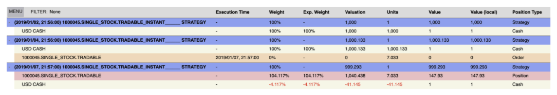
Overriding strategy execution time:
hours, minutes = 21, 56
decision_time = dtm.time(hours, minutes)
size_time = dtm.time(hours, minutes + 1)
execution_time = dtm.time(hours, minutes + 2)
Input:
decision_time
Output:
datetime.time(21, 56)
Input:
size_time
Output:
datetime.time(21, 57)
Input:
execution_time
Output:
datetime.time(21, 58)
local_zone = local_timezone.zone

rs_instant = sig.ReinvestmentStrategy(
    start_date=start_date,
    end_date=end_date,
    currency=stock_obj.currency,
    underlyer=ticker,
    withholding_tax_override=0.0,
    size_time_input=size_time,
    decision_time_input=decision_time,
    execution_time_input=size_time,
    size_timezone_input=local_zone,
    decision_timezone_input=local_zone,
    execution_timezone_input=local_zone,
    initial_shares=1,
    initial_cash=100,
    include_trading_costs=False,
    total_return=False,
)
rs_instant.build()
rs_instant.plot.portfolio_table(
    dts="TOP_ORDER_PTS",
    start_dt=start_date,
    end_dt=start_date + dtm.timedelta(days=10),
    tzinfo=local_timezone
)
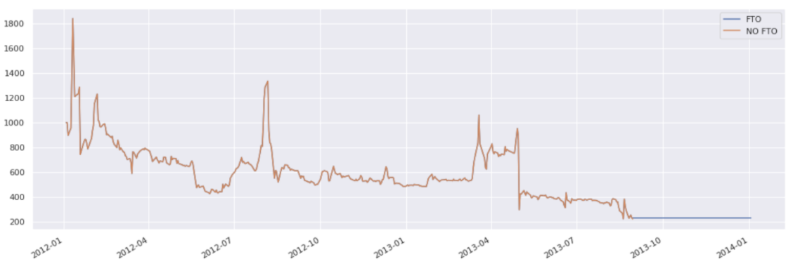
Trading out of stocks that will delist#
An example of a stock that was delisted due to bankruptcy:
Input:
delisted_stock_obj = sig.obj.get("1002181.SINGLE_STOCK.TRADABLE")
delisted_stock_obj.company_name
Output:
'EASTMAN KODAK'
Input:
delisted_stock_obj.expiry_date
Output:
datetime.date(2013, 8, 30)
Input:
delisted_stock_obj.delist_date
Output:
datetime.date(2013, 9, 3)
The final_trade_out parameter causes a Reinvestment Strategy to sell out of the underlying before it is delisted. The RS will then hold cash.
This can be very useful when another strategy, such as SignalStrategy, is trading a universe of RS. The onus will no longer be on you to ensure that no trades on the Reinvestment Strategy, corresponding to the delisted security, are initiated.
fto_start_date = dtm.date(2012, 1, 4)
fto_end_date = dtm.date(2014, 1, 4)
rs_no_fto = sig.ReinvestmentStrategy(
    start_date=fto_start_date,
    end_date=fto_end_date,
    currency=delisted_stock_obj.currency,
    underlyer=delisted_stock_obj.name,
    ticker=f"{delisted_stock_obj.name}_NO_FTO",
)
rs_no_fto.build()

rs_fto = sig.ReinvestmentStrategy(
    start_date=fto_start_date,
    end_date=fto_end_date,
    currency=delisted_stock_obj.currency,
    underlyer=delisted_stock_obj.name,

    # final trade out
    final_trade_out=True,

    ticker=f"{delisted_stock_obj.name}_FTO",
)
rs_fto.build()
The version of the RS with final_trade_out set to False has NaN prices from the delisting date onward, rendering it impossible to trade, which includes the closing of positions in it. The version with final_trade_out set to True does not have this problem.
df = pd.concat({
    "FTO": rs_fto.history(),
    "NO FTO": rs_no_fto.history(),
}, axis=1)
df.loc[delisted_stock_obj.expiry_date:].head()
df.plot()
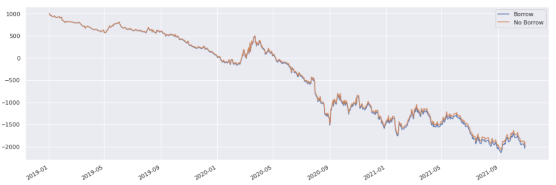
Borrow costs#
Shorting costs can be specified with the borrow_cost_ts parameter. The following example assumes there is no borrowing cost:
rs_short = sig.ReinvestmentStrategy(
    start_date=start_date,
    end_date=end_date,
    currency=stock_obj.currency,
    underlyer=ticker,
    ticker=f"{ticker}_RS_SHORT",

    # specific to shorting

    direction="short",
    # cash given opposite sign as we are short
    initial_cash=-1000,
    borrow_cost_ts=0,
    # should not specify dividend reinvestment when short
    reinvest_cash_dividends=False,
)
rs_short.build()
The following example uses a fixed annual cost of 1%:
Note: A time series could also be supplied.
rs_short_borrow = sig.ReinvestmentStrategy(
    start_date=start_date,
    end_date=end_date,
    currency=stock_obj.currency,
    underlyer=ticker,
    ticker=f"{ticker}_RS_SHORT_BORROW",

    # specific to shorting
    direction="short",
    # cash given opposite sign as we are short
    initial_cash=-1000,
    borrow_cost_ts=1,
    # should not specify dividend reinvestment when short
    reinvest_cash_dividends=False,
)
rs_short_borrow.build()

df = pd.concat({
    "Borrow": rs_short_borrow.history(),
    "No Borrow": rs_short.history(),
}, axis=1)
df.plot()
rs_short.plot.portfolio_table(
    dts="TOP_ORDER_PTS"
)
Trading in swap format#
Exposure to the underlying can also be obtained in swap format, with the relevant parameters being:
trade_swap_format: Equity traded as swap if set toTrue.swap_reset_frequency: Frequency at which swap is reset, which leads to margin cleanup.swap_include_financing: Financing, as determined by thelibor_instrument_nameandlibor_spreadparameters, is charged ifTrue.
rs_swap = sig.ReinvestmentStrategy(
start_date=start_date,
end_date=end_date,
currency=stock_obj.currency,
underlyer=ticker,
# swap specific parameters
trade_swap_format=True,
swap_reset_frequency='3M',
swap_include_financing=True,
reinvest_cash_dividends=False,
libor_instrument_name='US0003M INDEX',
libor_spread=0.001,
ticker=f'{ticker}_RS_SWAP_L3M',
)
rs_swap.build()
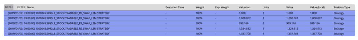
rs_swap.plot.portfolio_table(
dts='TOP_ORDER_PTS',
end_dt=dtm.date(2019, 4, 4),
tzinfo=local_timezone
)
Initial share holdings#
Create a Reinvestment Strategy that holds precisely one share and no cash. Transaction costs and accruals on cash are ignored.
rs_instant = sig.ReinvestmentStrategy(
    start_date=start_date,
    end_date=end_date,
    currency=stock_obj.currency,
    underlyer=ticker,

    initial_shares=1,
    initial_cash=0,
    total_return=False,
    include_trading_costs=False,

    ticker=f"{ticker}_RS_INITIAL1",
)
rs_instant.build()
rs_instant.plot.portfolio_table(
    dts="TOP_ORDER_PTS",
    end_dt=dtm.date(2019, 6, 30),
    tzinfo=local_timezone
)
A quick comparison with the output of calling adjusted_price_history:
df = pd.concat({
    "APH": stock_obj.adjusted_price_history(True, True),
    "RS": rs_instant.history()
}, axis=1).dropna().iloc[1:]
df /= df.iloc[0]
df.plot()
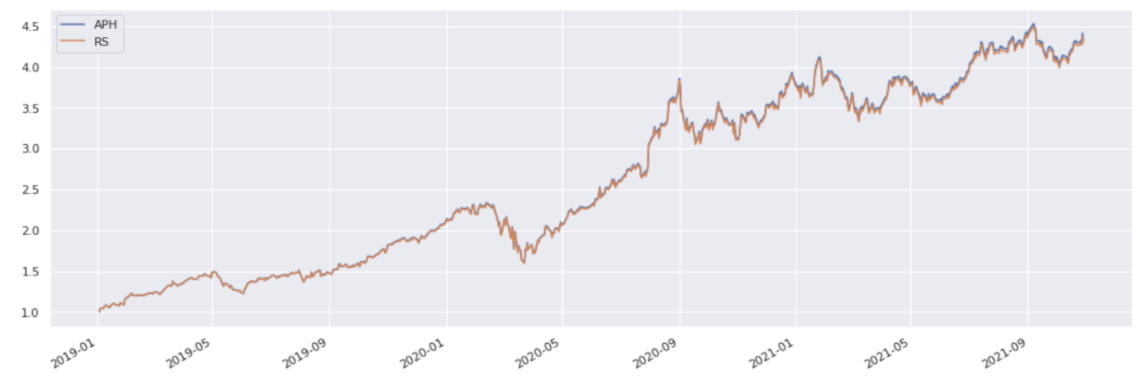
Input:
r = df.pct_change().dropna()
te = (r["APH"] - r["RS"]).std() * 16 * 100
print(f"Annualised TE versus Adjusted Price History: {round(te, 2)}%")
Output:
Annualised TE versus Adjusted Price History: 0.16%.
Comparing the ReinvestmentStrategy and Strategy classes#
Note: This section is optional reading.
By comparing the data_dict of an RS with its parent class, Strategy, we can see which of its arguments are unique to this building block.
Create a general Strategy object:
general_strategy = sig.Strategy(
    start_date=start_date,
    end_date=end_date,
    currency=stock_obj.currency
)
Access elements of the RS data_dict that are not present in the data_dict of a generic Strategy:
Input:
rs_only_keys = sorted([
    key for key in aapl_rs.data_dict()
    if key not in general_strategy.data_dict()
])
rs_only_keys
Output:
['borrow_cost_ts',
'corporate_actions_take_up_voluntary',
'enable_tracking', 'final_trade_out',
'initial_shares', 'libor_instrument_name',
'libor_spread', 'net_dividend_override',
'rebalance_bdc',
'rebalance_offset',
'rebalance_offset_sticky_end',
'reinvest_cash_dividends',
'spinoff_receive_cash',
'swap_include_financing',
'swap_reset_frequency',
'tracking_frequency',
'tracking_threshold',
'trade_swap_format',
'underlyer',
'underlyer_type',
'universe_filters',
'use_substrats',
'withholding_tax_override']