Bonds

Introduction

The purpose of this notebook is to show functionality related to bonds on the platform.

A notebook containing all the code used in this page can be accessed in the research environment: Example notebooks.

Environment

Setting up your environment takes three steps:

• Import the relevant internal and external libraries

• Configure the environment parameters

• Initialise the environment

import sigtech.framework as sig

import QuantLib as ql
import datetime as dtm
import seaborn as sns

sns.set(rc={'figure.figsize': (18, 6)})
sig.config.init();

Learn more: setting up the environment.

Government Bond Instrument

Government bonds are objects that can be retrieved by the object name constructed by the Country code, coupon, maturity date and ‘GOVT’ key.

bond_sig = sig.obj.get('US 2.625 2029/02/15 GOVT')

Each bond has various data elements accessible through their objects. The available time series for bond instruments are stored in the properties .history_fields and .extra_fields and are the following:

Python:

bond_sig.history_fields, bond_sig.extra_fields

Output:

(['AskPrice',
  'BidPrice',
  'LastPrice',
  'data_point',
  'HighPrice',
  'LowPrice',
  'MidPrice',
  'open',
  'open_interest',
  'Volume'],
 ['ModDuration', 'DV01', 'YTM'])

For querying the listed time series, the name of the time series can be passed in as the field parameter in the method .history(field = ) as shown below:

Python:

bond_sig.history(field='YTM').tail(5)

Output:

2021-04-26    0.013621
2021-04-27    0.014046
2021-04-28    0.014022
2021-04-29    0.014157
2021-04-30    0.014128
Name: (YTM, EOD, US 2.625 2029/02/15 GOVT), dtype: float64

Furthermore, the bond also holds relevant static data as seen below:

Python:

bond_sig.data_dict()

Output:

{'instrument_id': None,
 'data_source_all': [],
 'available_data_points': ['EOD'],
 'default_data_point': 'EOD',
 'price_factor': 1.0,
 'use_price_factor': True,
 'intraday_times': [],
 'intraday_tz_str': 'UTC',
 'currency': 'USD',
 'db_ticker': 'US 2.625 2029/02/15',
 'db_sector': None,
 'exchange_code': 'Unknown',
 'activity_fields': ['Volume'],
 'group_name': 'US GOVT BOND GROUP',
 'description': "2.625% NTS 15/02/2029 USD 'B-2029'",
 'coupon': 2.625,
 'coupon_type': 'FIXED',
 'coupon_frequency': 'SEMI_ANNUAL',
 'issue_date': datetime.date(2019, 2, 15),
 'issuer': 'United States Treasury Notes',
 'maturity_date': datetime.date(2029, 2, 15),
 'first_coupon_date': datetime.date(2019, 8, 15),
 'int_acc_date': datetime.date(2019, 2, 15),
 'redemption_amount': 100.0,
 'day_count': 'ACT/ACT',
 'isin': 'US9128286B18',
 'days_to_settle': 1,
 'first_settle_date': datetime.date(2019, 2, 15),
 'series_number': 'B-2029',
 'calc_type': 1,
 'db_history_end_date': datetime.date(9999, 12, 31),
 'country': 'US'}

Every single bond is part of a bond group, where a bond group contains all bonds issued by an issuer.

Python:

bond_group = bond_sig.group()
bond_group

Output:

US GOVT BOND GROUP <class 'sigtech.framework.instruments.bonds.BondGroup'>[5481449408]

As shown above, the bond group also acts as an object, therefore it holds functionality and data on its own. An example of the functionality is to query all bonds in a bond group which is shown below:

Python:

bond_group.query_instrument_names()[:5]

Output:

['US 0 2022/12/31 GOVT',
 'US 0.125 2013/08/31 GOVT',
 'US 0.125 2013/09/30 GOVT',
 'US 0.125 2013/12/31 GOVT',
 'US 0.125 2014/07/31 GOVT']

All coupons can be retrieved by the method .cashflows() as shown below:

Python:

bond_sig.cashflows(dtm.date(2021, 2, 1))

Output:

array([[datetime.date(2021, 2, 16), 1.3125000000000053, 0.0],
       [datetime.date(2021, 8, 16), 1.3125000000000053, 0.0],
       [datetime.date(2022, 2, 15), 1.3125000000000053, 0.0],
       [datetime.date(2022, 8, 15), 1.3125000000000053, 0.0],
       [datetime.date(2023, 2, 15), 1.3125000000000053, 0.0],
       [datetime.date(2023, 8, 15), 1.3125000000000053, 0.0],
       [datetime.date(2024, 2, 15), 1.3125000000000053, 0.0],
       [datetime.date(2024, 8, 15), 1.3125000000000053, 0.0],
       [datetime.date(2025, 2, 17), 1.3125000000000053, 0.0],
       [datetime.date(2025, 8, 15), 1.3125000000000053, 0.0],
       [datetime.date(2026, 2, 16), 1.3125000000000053, 0.0],
       [datetime.date(2026, 8, 17), 1.3125000000000053, 0.0],
       [datetime.date(2027, 2, 15), 1.3125000000000053, 0.0],
       [datetime.date(2027, 8, 16), 1.3125000000000053, 0.0],
       [datetime.date(2028, 2, 15), 1.3125000000000053, 0.0],
       [datetime.date(2028, 8, 15), 1.3125000000000053, 0.0],
       [datetime.date(2029, 2, 15), 1.3125000000000053, 100.0]],
      dtype=object)

Z-spread

The z-spread is calculated using the Python QuantLib library. Below is an example of when calculating the z-spread on a given date. For more information on the Python QuantLib library, see the Python QuantLib documentation.

bond_sig.z_spread(dtm.date(2020, 2, 28))

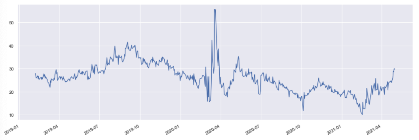
The z-spread can also be retrieved as a time series as shown below:

Python:

bond_sig.z_spreads().plot();

Output:

Asset swap spread

The asset swap spread is also calculated using the Python QuantLib library. The asset swap spread can be retrieved for a given date with the following method:

Python:

bond_sig.asw_spread(dtm.date(2020, 2, 28))

Output:

4.808005964045284

Convexity

Python:

ql_bond = bond_sig._quant_library_bond

ql.BondFunctions.convexity(
    ql_bond,
    0.05,
    ql_bond.dayCounter(),
    ql.Annual,
    ql_bond.frequency()
)

Output:

78.7683778608369

Modified duration

Python:

bond_sig.modified_duration(
    dtm.date(2020, 1, 4),
    6.
)

Output:

0.07241386265496533

Creating Strategies

To create strategies of forward contract, users can easily make use of the building block RollingBondStrategy object. For further information on RollingBondStrategy, see Rolling Bond Strategy.