Swaps#
Create and work with interest rate swaps. An interest rate swap is a derivative contract that involves the exchange of cash flows linked to fixed or floating interest rates over a period of time.
A notebook containing all the code used in this page can be accessed in the research environment: Example notebooks.
Environment#
Set up your environment using the following three steps:
Import the relevant internal and external libraries
Configure the environment parameters
Initialize the environment
import sigtech.framework as sig
from sigtech.framework.instruments.ir_otc import IRSwapMarket

import datetime as dtm
import pandas as pd
import numpy as np
import seaborn as sns
import matplotlib.pyplot as plt

sns.set(rc={'figure.figsize':(18,6)})
env = sig.init()
Learn more: Setting up your environment.
Interest Rate Swap Instrument#
Use InterestRateSwap to instantiate an interest rate swap. This class implements a receiver swap (receives fixed, pays floating) in which its profit and loss excluding cashflows is calculated from a given time series.
Compute the history of the swap by setting the value_post_start parameter to either of the following:
True: the swap’s history is computed to the earliest pricing day and swap maturity.False: the swap will only have time series from entry date until start date.
The example below shows the creation of a standard 6M EURIBOR IRS 30/360 semi annual receiver swap.
irs_std = sig.InterestRateSwap(
    currency='EUR',
    tenor='5Y',
    trade_date=dtm.date(2017, 1, 4),
    start_date=dtm.date(2017, 6, 20),
    value_post_start=True
    )
From this swap, various historic details are calculated. These are plotted below.
Input:
irs_std.floating_frequency
Output:
'6M'
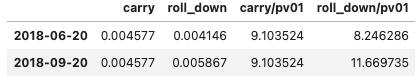
Use carry_roll_down to compute carry and roll-down of the swap by moving the valuation date forward.
Input:
irs_std.carry_roll_down(dtm.date(2017, 6, 20),
                        [dtm.date(2018, 6, 20), dtm.date(2018, 9, 20)])
Output:
Input:
irs_std.swap_details(dtm.date(2018, 4, 18), notional=250000000)
Output:
{'float_leg_pv': -2289013.305043739,
 'fixed_leg_pv': 2290709.7144424,
 'pv01': 125241.32304366023,
 'float_leg_pv_with_notional': -251495366.7555697,
 'fixed_leg_pv_with_notional': 251497063.16496837,
 'npv': 1696.4093986610549,
 'fixed_rate': 0.001829036662,
 'fair_rate': 0.0018276821494817399,
 'params': {'float_day_count': 'Actual/360',
  'fixed_day_count': '30/360 (Bond Basis)',
  'start_date': datetime.date(2017, 6, 20),
  'maturity': datetime.date(2022, 6, 20)},
 'fixed_flows': [(datetime.date(2018, 6, 20), 457259.1654999902),
  (datetime.date(2019, 6, 20), 457259.1654999902),
  (datetime.date(2020, 6, 22), 459799.49419722165),
  (datetime.date(2021, 6, 21), 455989.0011514023),
  (datetime.date(2022, 6, 20), 455989.0011514023)],
 'floating_flows': [(datetime.date(2018, 6, 20), -342513.8888888889),
  (datetime.date(2018, 12, 20), -323176.10197057924),
  (datetime.date(2019, 6, 20), -259151.09509436207),
  (datetime.date(2019, 12, 20), -87019.50997874742),
  (datetime.date(2020, 6, 22), 145395.57947229609),
  (datetime.date(2020, 12, 21), 436014.95916051336),
  (datetime.date(2021, 6, 21), 693461.8849646634),
  (datetime.date(2021, 12, 20), 917337.710956978),
  (datetime.date(2022, 6, 20), 1110030.9636272732)]}
The example below shows the creation of a 3M ERIBOR receiver swap (receives fixed, pays floating). Use the swap_details method to include the notional amount.
irs_3m = sig.InterestRateSwap(
    currency='EUR',
    tenor='10Y',
    trade_date=dtm.date(2017, 1, 4),
    start_date=dtm.date(2017, 6, 20),
    value_post_start=True,
    overrides={'forecast_curve':'EUR.F3M CURVE',
               'fixes_index':'EUR003M INDEX',  # What fixing to get
               'float_frequency': '3M', # This field determines the index tenor
              }
    )
Input:
irs_3m.floating_frequency
Output:
'3M'
Curves#
The interest rate swaps make use of historic forecasting and discounting curves.
Discounting methodology - LIBOR replacement#
Discounting is performed from standard curves, such as USD.D, EUR.D, and GBP.D.
For USD discounting, the curve is constructed from EFFR (Effective Fed Fund Rate) up to 18th Oct 2020. After this date it is replaced by SOFR (Secured Overnight Financing Rate) from 19th Oct 2020.
For EUR.D curve, EONIA (Euro OverNight Index Average) is the reference rate up to 26th Jul 2020. It is then replaced by ESTR (Euro Short-Term Rate) from 27th Jul 2020.
Input:
discounting_curve = sig.obj.get(IRSwapMarket.discounting_curve_name('USD'))

dt = pd.Timestamp(2019, 12, 30)
discounting_curve_history = discounting_curve.history()
discounting_curve_data = discounting_curve_history.loc[dt]
discounting_curve_df = pd.Series(discounting_curve_data)

discounting_curve_data.plot(
    title=discounting_curve.name + ' Discount Factors as of ' + str(dt)
);
Output:

Input:
discounting_curve.discount_factor(dtm.date(2020, 2, 3), dtm.date(2020, 3, 3))
Output:
0.9987149786544263
Input:
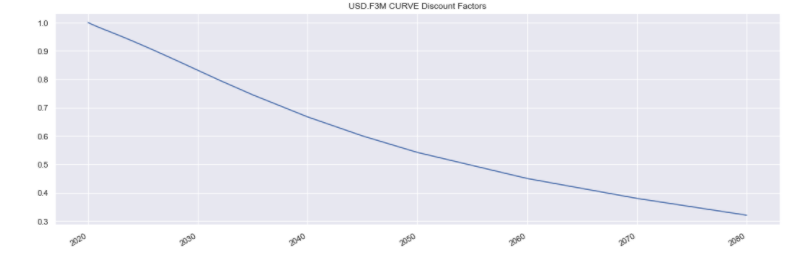
forecasting_curve = sig.obj.get(IRSwapMarket.forecasting_curve_name('USD'))

dt = pd.Timestamp(2019, 12, 30)
forecasting_curve_history = forecasting_curve.history()
forecasting_curve_data = forecasting_curve_history.loc[dt]

forecasting_curve_df = pd.Series(
    index=forecasting_curve_data['Dates'],
    data=forecasting_curve_data['DiscountFactors']
)

forecasting_curve_df.plot(title=forecasting_curve.name + ' Discount Factors');
Output:
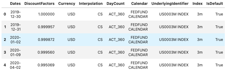
Below is the forecasting curve as a table:
Input:
pd.DataFrame(forecasting_curve_data).head()
Output:
Below is an example of how to retrieve the raw values of the projection curve:
Input:
raw_data = env.data_service.projection_curve(
    'USD.F3M CURVE',
    fields=['LastPrice'],
    data_point='EOD'
)
raw_values = pd.Series(raw_data.iloc[8].values[0])
raw_values
Output:
Depos            {'1d': 4.29875, '2d': 4.31576, '1w': 4.31938, ...
Futures          {'mar-2006': 95.2425, 'jun-2006': 95.1875, 'se...
Convexity        {'mar-2006': 0.0001, 'jun-2006': 0.0004, 'sep-...
Fras                                                            {}
Swaps            {'1y': 4.83, '2y': 4.794, '3y': 4.788, '4y': 4...
SwapFrequency    {'1y': 'Annual', '2y': 'Semi Annual', '3y': 'S...
SwapDayCounts    {'1y': 'ACT_360', '2y': '30_360', '3y': '30_36...
dtype: object
The performance of a swap over time can be retrieved via the history() method. The relevant time series data fields for a swap are the following:
Input:
irs_std.history_fields
Output:
['LastPrice', 'Rate', 'PV01']
Generate the rate as a time series:
Input:
rate = pd.concat({
    '6M Euribor Swap Rate': irs_std.history('Rate'),
    '3M Euribor Swap Rate': irs_3m.history('Rate')}, axis=1)
rate.iloc[0]
Output:
6M Euribor Swap Rate    0.173544
3M Euribor Swap Rate    0.666249
Name: 2017-01-03 00:00:00, dtype: float64
Generate the net present value as a time series:
Input:
npv = pd.concat({
    '6M Euribor Swap NPV': irs_std.history('LastPrice'),
    '3M Euribor Swap NPV': irs_3m.history('LastPrice')}, axis=1)
npv.iloc[0]  # value per unit
Output:
6M Euribor Swap NPV    0.000471
3M Euribor Swap NPV    0.001303
Name: 2017-01-03 00:00:00, dtype: float64
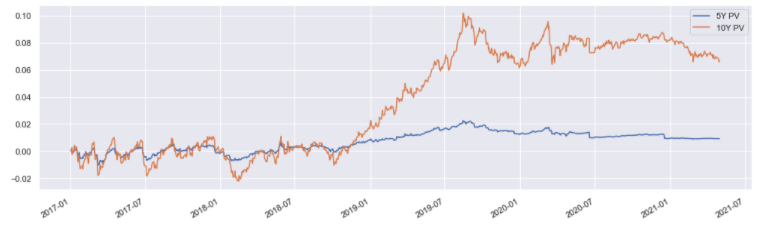
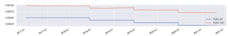
Below is an example of how to create a 5s10s steepener:
irs_std_10y = sig.InterestRateSwap(
    currency='EUR',
    tenor='10Y',
    trade_date=dtm.date(2017, 1, 4),
    start_date=dtm.date(2017, 6, 20),
    value_post_start=True
)
s5s10s = pd.concat({
    '5Y PV': irs_std.history(),
    '10Y PV': irs_std_10y.history(),
    'PV01 5Y': irs_std.history('PV01'),
    'PV01 10Y': irs_std_10y.history('PV01')}, axis=1)
Input:
s5s10s[['5Y PV','10Y PV']].plot(figsize=(17, 5))
Output:
Input:
s5s10s[['PV01 5Y','PV01 10Y']].plot(figsize=(17, 2))
Output:
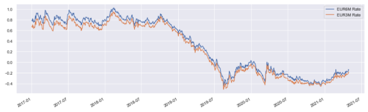
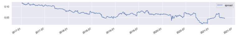
Below is an example of how to visualize the basis between different tenors:
rate = pd.concat({
    'EUR6M Rate': irs_std_10y.history('Rate'),
    'EUR3M Rate': irs_3m.history('Rate')}, axis=1)
rate['spread'] = rate['EUR6M Rate'] - rate['EUR3M Rate']
Input:
rate.iloc[:, :2].plot(figsize=(17, 5))
Output:
Input:
rate.iloc[:, -1:].plot(figsize=(17, 2))
Output:
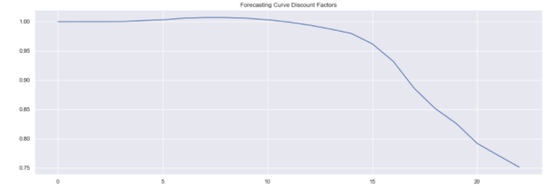
Shifting Valuation Date#
The quant library allows the rate spread to be determined between two dates, keeping the curve fixed.
The examples below give a forecasted curve fcst_curve and a discounted curve disc_curve.
Input:
pds = pd.Series(fcst_curve.history().loc[dt].get('DiscountFactors')).plot(
    title='Forecasting Curve Discount Factors');
Output:
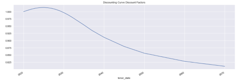
Input:
disc_curve.history().loc[dt].plot(title='Discounting Curve Discount Factors');
Output:
Historic Swap Rates#
Use the curve history to evaluate the swap rates for various tenors throughout the history. You can retrieve a single tenor historical time series and forward starting fair swap rates.
When initializing an InterestRateSwapGroup, use the tenor parameter to change the period.
Input:
print(sig.obj.get('USD.D CURVE').get_swap_rate('5Y'))
Output:
	          5Y
trading_datetime
2006-01-02	4.44865
2006-01-03	4.31762
2006-01-04	4.31263
2006-01-05	4.31150
2006-01-06	4.30889
Input:
print(sig.InterestRateSwapGroup.fair_rate_df(currency='USD',
                                     tenor='3Y',
                                     fwd_tenor='2Y',
                                     start_date=dtm.date(2010,2,3)
                                    ))
Output:
            Rate 2Yx3Y  PV01 2Yx3Y  PnL 2Yx3Y
2010-02-03    3.829934    0.000278        NaN
2010-02-04    3.711822    0.000279   0.003481
2010-02-05    3.652153    0.000280   0.001668
2010-02-08    3.643886    0.000280   0.000362
2010-02-09    3.736597    0.000279  -0.002552
...                ...         ...        ...
2024-11-20    4.090634    0.000259  -0.000154
2024-11-21    4.112500    0.000259  -0.000568
2024-11-22    4.087089    0.000259   0.000657
2024-11-25    3.966415    0.000260   0.003129
2024-11-26    3.966389    0.000260  -0.000002
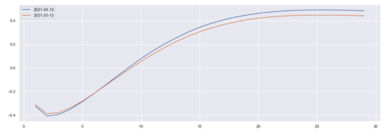
You have the option to change the interpolation method—see below.
Input:
dts = forecasting_curve.history().loc[dtm.date(2010, 2, 1):].index
swap_crv = {}
for d in dts[21::21]:
    try:
        swp = pd.Series(data=[sig.InterestRateSwap.fair_rate_df(
            env, 'EUR', str(x) + 'Y', d)
            for x in range(1, 30)], index=list(range(1, 30)))
        swap_crv[d.date()] = swp
    except:
        pass

swap_rates = 100 * pd.concat(swap_crv, axis=1).iloc[::-1]

swap_rates.interpolate('spline',order=3).iloc[:,-1].plot()
swap_rates.interpolate('spline',order=3).iloc[:,-2].plot()
plt.legend()
Output:
Overnight Index Swap Instrument#
Representing a single overnight index swap (OIS) contract, the OISSwap class receives fixed rate and pays OIS rate. The OISSwapGroup class represents a group of OIS contracts, and can be used to manage multiple OIS swaps that share common characteristics.
The example below instantiates an overnight interest rate swap with different payment frequencies:
from sigtech.framework.instruments.ois_swap import OISSwap

ois_q = OISSwap(currency='USD',
               tenor='10Y',
               start_date=dtm.date(2016, 7, 5),
               frequency = 'Q')

ois_a = OISSwap(currency='USD',
                tenor='10Y',
                start_date=dtm.date(2016, 7, 5),
                frequency = 'A')

ois_s = OISSwap(currency='USD',
                tenor='10Y',
                start_date=dtm.date(2016, 7, 5),
                frequency = 'SA')
The performance of a swap over time can be retrieved via the history method. You can also use history_fields to obtain a list of relevant time series data fields for a swap—see below:
Input:
ois_a.history_fields
Output:
['LastPrice', 'FairRate', 'PV01']