Size a rolling future strategy

Size rolling future strategies with initial cash or fixed contracts, and compare the different sizing methods.

• Initial cash sizing (Default): The strategy uses its initial cash to buy as many futures contracts as possible. If no initial_cash parameter is provided, the strategy assumes 1000 currency units.

• Fixed number of contracts sizing: Overwrite the default sizing so that a fixed number of contracts is always traded, independent of the initial_cash amount.

Size a rolling future strategy with initial cash

In this example the strategy initially buys as many future contracts as possible using the initial_cash.

Calculate the cash required to buy 100 contracts of crude oil futures:

START_DATE = dtm.date(2023, 1, 1)
PREVIOUS_DAY = dtm.date(2022, 12, 31)
END_DATE = dtm.date(2024, 1, 1)

n_contracts = 100

co = sig.obj.get("CO COMDTY FUTURES GROUP")
contract = co.contract_instruments(PREVIOUS_DAY, PREVIOUS_DAY)[0]
price_t = contract.history()["2022-12"][-1]
initial_cash = contract.contract_size * n_contracts * price_t
initial_cash

To examine mark-to-market profit and loss, exclude trading costs and cash interest accrual.

co_strat = sig.RollingFutureStrategy(
    start_date=START_DATE,
    end_date=END_DATE,
    currency="USD",
    contract_code="CO",
    contract_sector="COMDTY",
    rolling_rule="front",
    front_offset="-5,-3",
    include_trading_costs=False,
    total_return=False,  # don't include cash accrual
    set_weight_from_initial_cash=True,
    initial_cash=initial_cash,
)
history_series = co_strat.history()
print(history_series.tail())
history_series.plot()

In the example above, the strategy’s history is the mark-to-market profit and loss.

To reconcile the calculations, use the price_series method to get a simple series of price data:

price_series = co_strat.price_series()

Calculate the mark-to-market with the following formula:

\[\mathrm{PnL} = \mathrm{ContractSize} \times \mathrm{NContracts} \times \mathrm{Price}_{chng}\]

where:

• \(\mathrm{ContractSize}\) is the notional of the future contract

• \(\mathrm{NContracts}\) is the number of contracts held

• \(\mathrm{Price}_{chng}\) is the price difference from t to t+1

price = co_strat.price_series()
print(price.head())
price.plot();

print('MtM\n', initial_cash + (price.diff().head(8) * co.contract_size * n_contracts))
print('----')
print('history\n', co_strat.history()[2:9])

Output:

MtM
 2017-03-03          NaN
2017-03-06    5519000.0
2017-03-07    5499000.0
2017-03-08    5227000.0
2017-03-09    5416000.0
2017-03-10    5426000.0
2017-03-13    5506000.0
2017-03-14    5465000.0
dtype: float64
----
history
 2017-03-06    5519000.0
2017-03-07    5510000.0
2017-03-08    5229000.0
2017-03-09    5137000.0
2017-03-10    5055000.0
2017-03-13    5053000.0
2017-03-14    5010000.0

The strategy sizing is based on the available cash and the price of the futures instrument. This means that the number of futures contracts traded can vary.

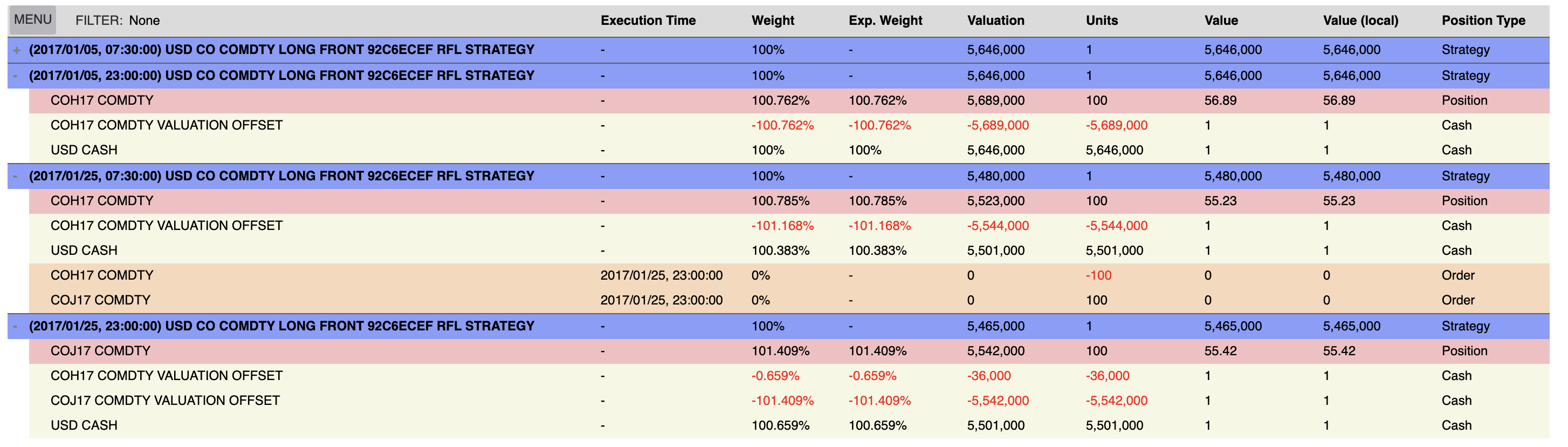
To verify the strategy results and sizing, use the portfolio_table method in the sig.Strategy.plot utility wrapper:

co_strat.plot.portfolio_table(
    'TOP_ORDER_PTS',
    start_dt=start_date,
    end_dt=start_date+dtm.timedelta(days=30),
    unit_type='TRADE') # shows the portfolio in number of contracts

The strategy’s initial cash is based on the previous day’s price data.

You might see what seems to be a slight discrepancy between the initial cash calculation and the strategy results. This is because the strategy’s history is based on the price data available at execution time.

Size a rolling future strategy with a fixed number of contracts

You can also size a rolling future strategy by specifying a fixed number of futures contracts to trade:

co_fixed_sizing = sig.RollingFutureStrategy(
    currency='USD',
    start_date=start_date,
    contract_code='CO',
    contract_sector='COMDTY',
    rolling_rule='front',
    front_offset='-5:-4',
    include_trading_costs=False,
    total_return=False, # don't include cash accrual
    set_weight_from_initial_cash=True,
    initial_cash=initial_cash,
    fixed_contracts=100.0,
)

Verify that the fixed contract strategy is rolling 100 contracts:

co_fixed_sizing.plot.portfolio_table(
    'TOP_ORDER_PTS',
    start_dt=start_date,
    end_dt=start_date+dtm.timedelta(days=30),
    unit_type='TRADE'
)

Plot the performance of both strategies:

sig.PerformanceReport([co_fixed_sizing, co_strat]).report()