Options#

This page shows how individual options and volatility surfaces work on the platform.

Environment#

Setting up your environment takes three steps:

Import the relevant internal and external libraries
Configure the environment parameters
Initialize the environment

import sigtech.framework as sig

import datetime as dtm
import pandas as pd
import seaborn as sns

sns.set(rc={'figure.figsize': (18, 6)})
sig.config.init()

Learn more: Setting up the environment

Vanilla Options#

Overview#

To create a vanilla option on the SigTech platform, carry out the following steps:

1) Get option group#

The available option groups can be viewed in the Data Browser. To retrieve an option group, use the following syntax and insert the relevant option group name:

option_group = sig.obj.get('<Insert Relevant Option Group Name>')

2) Create option#

Retrieve the option by calling the .get_option() method on the option group object. Below is an example:

option = option_group.get_option(
    option_type='Call',
    strike=1100,
    start_date=dtm.date(2010, 4, 6),
    maturity=dtm.date(2011, 4, 6)
)

If you’re getting an option for a futures group (such as CO COMDTY OTC OPTION GROUP) the maturity date must match an expiration date of one of the futures in the group. To find a valid maturity date that is closest to a given a date, use the following method: option.available_maturity(dtm.date(2011,4,6)).

Example: Index OTC option#

An index over-the-counter (OTC) option gives you the right to buy or sell the value of an index at a specified price.

On the SigTech platform, use sig.obj.get to retrieve the option group. You can then create the option instrument.

Input:

# Get the option group
equity_option_group = sig.obj.get('SPX INDEX OTC OPTION GROUP')

# Create the option
spx_call_option = equity_option_group.get_option(
    option_type='Call',
    strike=1100,
    start_date=dtm.date(2010, 4, 6),
    maturity=dtm.date(2011, 4, 6)
)
spx_call_option

Output:

SPX 20110406 CALL 1100 604506EC INDEX <class 'sigtech.framework.instruments.options.EquityIndexOTCOption'>[4534898352]

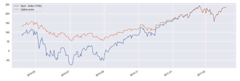
You can also plot the valuation of each option. This is compared below to the underlying asset minus the strike.

pd.concat({
    'Spot - strike (1100)': spx_call_option.underlying_object.history() - 1100,
    'Option price': spx_call_option.history()
}, axis=1).dropna().plot();

Example: FX OTC option#

The FXOTCOptionsGroup class represents FX OTC option groups.

Use the get_group method to retrieve the option group, then create the FX OTC option:

eur_usd_group = sig.FXOTCOptionsGroup.get_group('USDEUR')

eurusd_call_option = eur_usd_group.get_option('Call', 1.3, dtm.date(2010, 4, 6),
                                              dtm.date(2011, 4, 6))

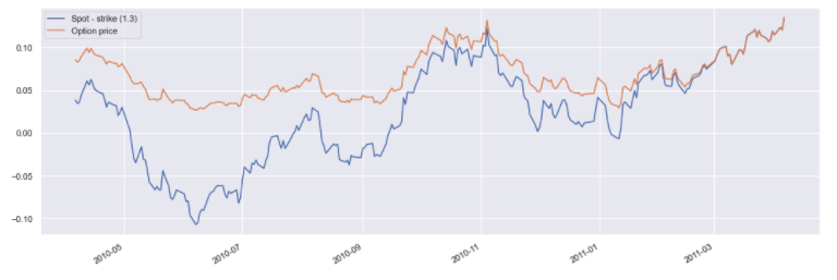
Plot the valuation:

pd.concat({
    'Spot - strike (1.3)': eurusd_call_option.underlying_object.history() - 1.3,
    'Option price': eurusd_call_option.history()
}, axis=1).dropna().plot();

Other OTC option groups#

As well as FXOTCOptionsGroup above, other OTC option group classes include:

OTCOptionGroup
EquityIndexOTCOptionsGroup
CommodityOTCOptionsGroup
ETFOTCOptionsGroup
FXOTCOptionsGroup
VolatilityIndexOTCOptionsGroup

You can use these option group classes to create the corresponding option. To view a list of available options, use the get_names method—the example below retrieves a list of ETF OTC options:

sig.instruments.option_groups.ETFOTCOptionsGroup.get_names(include_children=True)

Alternative way of creating options#

Options can also be created explicitly from an option class without using the option group. Some of the option classes available include:

`EquityIndexOTCOption`#

This class implements OTC equity index option instruments.

Input:

equity_option = sig.EquityIndexOTCOption(
    currency='USD',
    maturity_date=dtm.date(2011, 4, 6),
    option_type='Call',
    start_date=dtm.date(2010, 4, 6),
    strike=1100,
    underlying='SPX INDEX',
)
equity_option

Output:

SPX 20110406 CALL 1100 A6D17D99 INDEX <class 'sigtech.framework.instruments.options.EquityIndexOTCOption'>[5966872832]

`FXOTCOption`#

This class implements FX OTC option instruments. Parameters include:

over: The over currency of the underlying pair (e.g. USD for EURUSD)
under: The under currency of the underlying pair (e.g. EUR for EURUSD)

Use FXOTCOption to create the instrument:

instr = sig.FXOTCOption(
    over='USD',
    under='EUR',
    strike=1.0635,
    start_date=dtm.date(2017, 1, 6),
    maturity_date=dtm.date(2017, 4, 6),
    option_type='Call'
)

`CommodityFutureOTCOption`#

This class implements OTC commodity future options:

instr = sig.CommodityFutureOTCOption(
    currency='USD',
    start_date=dtm.date(2018, 8, 22),
    strike=80,
    maturity_date=dtm.date(2019, 1, 28),
    option_type='Put',
    underlying='COH19 COMDTY',
    exercise_type='American'
)

`CommodityFutureOTCDigitalOption`#

This class implements OTC commodity future digital options. A digital option is a type of option that lets you manually set a strike price. You receive a fixed payout when the market price of the underlying asset exceeds the strike price.

Create the instrument:

instr = sig.CommodityFutureOTCDigitalOption(
    currency='USD',
    start_date=dtm.date(2018, 7, 22),
    strike=75,
    maturity_date=dtm.date(2019, 1, 28),
    underlying='COH19 COMDTY'
)

Exotic options#

Overview#

When dealing with other options apart from vanilla options, it’s easy to modify the .get_options() method depending on use case. The available exotic options are:

Digital
Barriers (KO & KI)
One-touch & no-touch

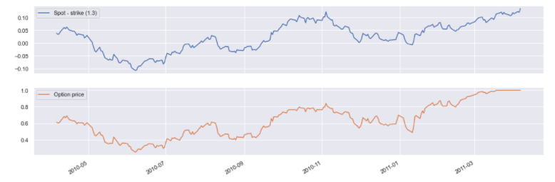
Digital #

digital = eur_usd_group.get_option('Call', 1.3, dtm.date(2010, 4, 6),
                                   dtm.date(2011, 4, 6), digital=True)

pd.concat({
    'Spot - strike (1.3)': digital.underlying_object.history() - 1.3,
    'Option price': digital.history()
}, axis=1).dropna().plot(subplots=True);

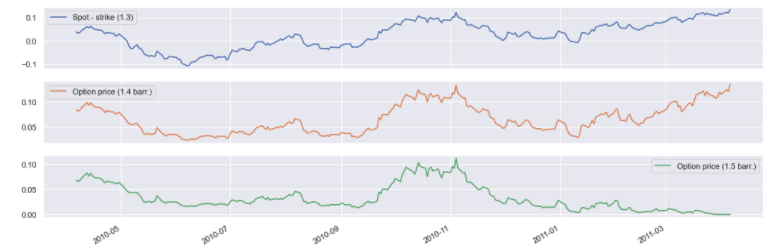
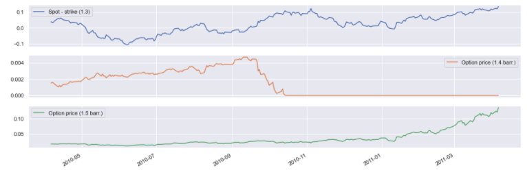
Barriers: KO & KI #

ki_barrier_1 = eur_usd_group.get_option('Call', 1.3,
                                        dtm.date(2010, 4, 6), dtm.date(2011, 4, 6),
                                        barrier_type='KI', barrier=1.5)
ki_barrier_2 = eur_usd_group.get_option('Call', 1.3,
                                        dtm.date(2010, 4, 6), dtm.date(2011, 4, 6),
                                        barrier_type='KI', barrier=1.4)

pd.concat({
    'Spot - strike (1.3)': ki_barrier_1.underlying_object.history() - 1.3,
    'Option price (1.4 barr.)': ki_barrier_2.history(),
    'Option price (1.5 barr.)': ki_barrier_1.history()
}, axis=1).dropna().plot(subplots=True);

ko_barrier_1 = eur_usd_group.get_option('Call', 1.3,
                                        dtm.date(2010, 4, 6), dtm.date(2011, 4, 6),
                                        barrier_type='KO', barrier=1.5)
ko_barrier_2 = eur_usd_group.get_option('Call', 1.3,
                                        dtm.date(2010, 4, 6), dtm.date(2011, 4, 6),
                                        barrier_type='KO', barrier=1.4)

pd.concat({
    'Spot - strike (1.3)': ko_barrier_1.underlying_object.history() - 1.3,
    'Option price (1.4 barr.)': ko_barrier_2.history(),
    'Option price (1.5 barr.)': ko_barrier_1.history()
}, axis=1).dropna().plot(subplots=True);

One-touch & no-touch #

ot_barrier = eur_usd_group.get_option('Call', 1.4,
                                      dtm.date(2010, 4, 6), dtm.date(2011, 4, 6),
                                      barrier_type='OT', digital=True)
nt_barrier = eur_usd_group.get_option('Call', 1.4,
                                      dtm.date(2010, 4, 6), dtm.date(2011, 4, 6),
                                      barrier_type='NT', digital=True)

pd.concat({
    'Spot - strike (1.3)': ot_barrier.underlying_object.history() - 1.3,
    'Option price (One-touch 1.4)': ot_barrier.history(),
    'Option price (No-touch 1.4)': nt_barrier.history()
}, axis=1).dropna().plot(subplots=True);

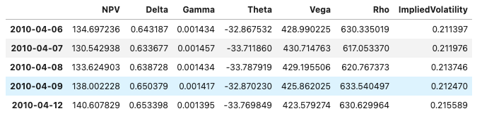
Greeks#

The Greeks for each option can be queried in the following way:

equity_option.option_metrics().head()

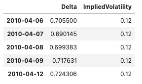
The volatility can be overwritten in the Greeks calculation. This override can be specified as a float or time series of vols.

equity_option.option_metrics(
    fields=['Delta', 'ImpliedVolatility'], vol_override=0.12).head()

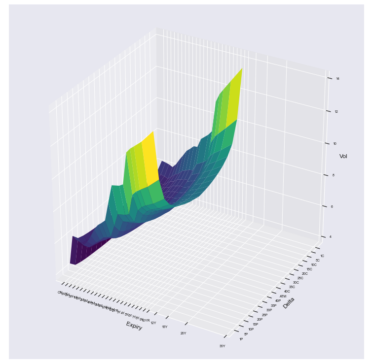
Vol surface #

Retrieve vol surface object #

Input:

vs = sig.obj.get('EURUSD VOLSURFACE')
vs

Output:

EURUSD VOLSURFACE <class 'sigtech.framework.infra.vol_surfaces.vol_surface.FXVolSurface'>[5572896224]

vs.plot_surface(d=vs.history_dates_actual()[-1], z_name='Vol')

get_vol based on the effective date, expiry date and strike.

Input:

vs.get_vol(dtm.date(2019, 3, 29), dtm.date(2019, 4, 28), 1.34)

Output:

0.05693914182317497

Vol surface iterator#

The FXVolSurfaceIterator class simplifies the retrieval of a set of volatility surfaces for a selection of currencies and associated data.

Input:

vol_iterator = sig.FXVolSurfaceIterator(['USD', 'EUR', 'GBP'])
list(vol_iterator.iterate_surfaces())

Output:

[EURUSD VOLSURFACE <class 'sigtech.framework.infra.vol_surfaces.vol_surface.FXVolSurface'>[5572896224],
 GBPUSD VOLSURFACE <class 'sigtech.framework.infra.vol_surfaces.vol_surface.FXVolSurface'>[5973002656],
 EURGBP VOLSURFACE <class 'sigtech.framework.infra.vol_surfaces.vol_surface.FXVolSurface'>[5981535392]]

Use the iterator class to generate a list of all available surfaces:

Input:

sig.FXVolSurfaceIterator.get_all_available_surfaces_names()[:5]

Output:

['AUDBRL VOLSURFACE',
 'AUDCAD VOLSURFACE',
 'AUDCHF VOLSURFACE',
 'AUDCNH VOLSURFACE',
 'AUDHKF VOLSURFACE']

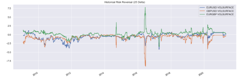
Using the FXVolSurfaceIterator instance, you can obtain the historical implied ATM volatilities and risk reversals:

implied_1m_vol_history_df = vol_iterator.atm_vols_for_tenor('1M')
implied_1m_vol_history_df.plot(title='Historical Implied Volatilities');

rr_history_df = vol_iterator.risk_reversal('1M', 25)
rr_history_df.plot(title='Historical Risk Reversal (25 Delta)');

The available tenors can be listed with the get_all_available_tenors method:

Input:

vol_iterator.get_all_available_tenors()[:10]

Output:

['-', 'O/N', 'ON', '1W', '1WK', '2WK', '2W', '3WK', '3W', '1M']

Table of Contents

Options

Options#

Environment#

Vanilla Options#

Overview#

1) Get option group#

2) Create option#

Example: Index OTC option#

Example: FX OTC option#

Other OTC option groups#

Alternative way of creating options#

EquityIndexOTCOption#

FXOTCOption#

CommodityFutureOTCOption#

CommodityFutureOTCDigitalOption#

Exotic options#

Overview#

Digital #

Barriers: KO & KI #

One-touch & no-touch #

Greeks#

Vol surface #

Retrieve vol surface object #

Vol surface iterator#

`EquityIndexOTCOption`#

`FXOTCOption`#

`CommodityFutureOTCOption`#

`CommodityFutureOTCDigitalOption`#