Swaptions#
Introduction#
A swaption is an option to enter an interest rate swap at some point in the future, on the swaption expiry date.
There are two types of swaption:
Payer swaption: An option to enter into a swap as a fixed-rate payer.
Receiver swaption: An option to enter into a swap as a fixed-rate receiver.
The fixed rate of the swap is determined by the strike of the swaption.
Example: A 3Mx5Y 2% receiver swaption gives the holder the right to enter into a 5 year swap, starting 3 months after the swaption start date, and receiving a 2% fixed rate whilst paying a floating (LIBOR) rate according to the usual currency conventions.
Settlement#
A Swaption can be settled in cash, or in a physical swap. The style of the settlement is determined by the swaption currency. All currencies in the SigTech framework assume a physical settlement, with the exception of GBP and EUR.
Previously, cash settlement was calculated as a function of the swap par (forward) rate. As of 26 November 2018, EUR swaptions have been settled at the fair value for standard collateralised EUR swaps and are, as far as valuation is concerned, indistinguishable from physically settled swaptions.
If the swaption survives to the exercise date and is in the money, it is settled physically for USD but in cash for EUR. GBP swaptions continue to use the swap rate based formula.
Modelling & pricing#
Swaptions use the normal model. As rates are generally close to zero, and can even be negative, the log-normal assumption used for options is inappropriate.
Some market participants use a shifted log-normal model, where instead of an underlying rate of r, a shifted rate is applied, such as r+2%. Such an approach assumes that the process is log-normal.
Environment#
Setting up your environment takes three steps:
Import the relevant internal and external libraries
Configure the environment parameters
Initialize the environment
import sigtech.framework as sig

import datetime as dtm
import pandas as pd
import seaborn as sns

sns.set(rc = {"figure.figsize": (18, 6)})

if not sig.config.is_initialised():
    env = sig.init()
Learn more: Setting up the environment
SABR#
The SABR model is a stochastic volatility model which attempts to capture the volatility smile in derivatives markets. The model is widely used by participants in interest rate derivative markets. The standard approach when interpolating swaption volatilities is to first calibrate the SABR parameters, keeping expiry and swap tenor constant, varying the strikes, and then using them to recover the volatilities.
To price an option with a tenor existing on the (SABR) volatility surface, the normal volatility from parameters is inferred, and is used as a Bachelier (normal) pricer. If the expiry is not part of the surface, the corresponding normal volatilities for neighbouring tenors is found on the surface and linearly interpolate between them.
To view all tenors for a particular currency, the following code block can be used:
Input:
single_surface = sig.obj.get("USD SWAPTION SABR VOLSURFACE").get_handle(dtm.date(2021,11,10))
single_surface.market_quotes["Tenor"].squeeze().unique()
Output:
[10Y, 15Y, 1Y, 20Y, 25Y, ..., 5Y, 6Y, 7Y, 8Y, 9Y]
Length: 14
Categories (14, object): [10Y, 15Y, 1Y, 20Y, ..., 6Y, 7Y, 8Y, 9Y]
The following call will give all the (currency) SABR parameters for a given date:
Input:
single_surface.market_quotes
Output:
Field	Tenor	Expiry_date	Expiry	Alpha	Beta	Rho	Nu	Shift
data_point	NEW_YORK_1600	NEW_YORK_1600	NEW_YORK_1600	NEW_YORK_1600	NEW_YORK_1600	NEW_YORK_1600	NEW_YORK_1600	NEW_YORK_1600
internal_id	USD SWAPTION SABR VOLSURFACE	USD SWAPTION SABR VOLSURFACE	USD SWAPTION SABR VOLSURFACE	USD SWAPTION SABR VOLSURFACE	USD SWAPTION SABR VOLSURFACE	USD SWAPTION SABR VOLSURFACE	USD SWAPTION SABR VOLSURFACE	USD SWAPTION SABR VOLSURFACE
Tenor	Expiry_date
10Y	2031-11-10	10Y	2031-11-10	10Y	0.017575	0.35	-0.052354	0.240327	0.03
15Y	2031-11-10	15Y	2031-11-10	10Y	0.016919	0.35	-0.081109	0.238704	0.03
1Y	2031-11-10	1Y	2031-11-10	10Y	0.019121	0.35	0.054083	0.244490	0.03
20Y	2031-11-10	20Y	2031-11-10	10Y	0.016395	0.35	-0.106717	0.237052	0.03
25Y	2031-11-10	25Y	2031-11-10	10Y	0.016097	0.35	-0.130014	0.236156	0.03
...	...	...	...	...	...	...	...	...	...
5Y	2030-11-08	5Y	2030-11-08	9Y	0.019030	0.35	0.035291	0.246928	0.03
6Y	2030-11-08	6Y	2030-11-08	9Y	0.018818	0.35	0.019300	0.246869	0.03
7Y	2030-11-08	7Y	2030-11-08	9Y	0.018602	0.35	0.005006	0.247866	0.03
8Y	2030-11-08	8Y	2030-11-08	9Y	0.018391	0.35	-0.009620	0.248066	0.03
9Y	2030-11-08	9Y	2030-11-08	9Y	0.018215	0.35	-0.023850	0.249120	0.03
Framework functionality#
In the SigTech framework, a swaption can be constructed directly from sig.Swaption() or by using a group get_swaption() function.
You can get the group using sig.SwaptionGroup.get_group("USD"). Expiry can be passed as a date or as a tenor. Strike can be numerical or offset in basis points from an at-the-money (ATM) forward.
Note: ATM is the equivalent of forward. ‘ATM+25bp’ is forward plus 0.0025 basis points.
The following command can be used to retrieve the docstrings associated with the swaption class:
sig.Swaption?
To retrieve the SwaptionGroup, use the get_group function:
usd_swaption_group = sig.SwaptionGroup.get_group("USD")
This group name can then be passed into sig.Swaption() when building your instrument:
s = sig.Swaption(
        start_date=dtm.date(2019, 12, 19),
        strike="ATM+10bp",
        expiry="3M",
        swap_tenor="5Y",
        option_type="Receiver",
        swaption_group=usd_swaption_group.name,
        currency="USD"
    )
The history for our swaption is then tabulated:
Input:
s.history()
Output:
2019-12-19    0.008366
2019-12-20    0.008170
2019-12-23    0.007511
2019-12-24    0.008018
2019-12-27    0.009359
                ...
2020-03-13    0.051148
2020-03-16    0.060423
2020-03-17    0.050462
2020-03-18    0.050184
2020-03-19    0.054498
Name: (NPV, EOD, USD 0.0181766 2019-12-19 2020-03-19X5Y REC SWAPTION), Length: 63, dtype: float64
OIS swaptions#
This class represents a swaption with an overnight indexed swap (OIS) as an underlying asset. All the parameters and functions are the same as the parent Swaption class.
Here’s an example of how to create an OIS swaption in the SigTech platform:
ois_swaption = sig.OISSwaption(
    start_date=dtm.date(2022, 2, 3),
    expiry="3M",
    swap_tenor="5Y",
    option_type="Payer",
    strike="ATM",
    currency="USD"
)
Spot vs forward premium#
All swaptions in the framework are modelled using spot premium as default. Spot premium refers to when payment occurs at the time of entering the contract. This can be contrasted with the forward premium which refers to when payment occurs at the time of exercising the option. A forward premium implies that no initial payment, or spot premium, for the swaption is made.
This can be modeled by setting forward_premium to True, which automatically infers a forward premium from the swaption value. Or, forward_premium can be set to the actual pre-agreed premium, so that it is taken into account when retrieving the resulting swaption’s present value and Greeks.
s_fp = sig.Swaption(
        start_date=dtm.date(2019, 12, 19),
        strike="ATM+10bp",
        expiry="3M",
        swap_tenor="5Y",
        option_type="Receiver",
        swaption_group=usd_swaption_group.name,
        currency="USD",
        forward_premium = True
    )
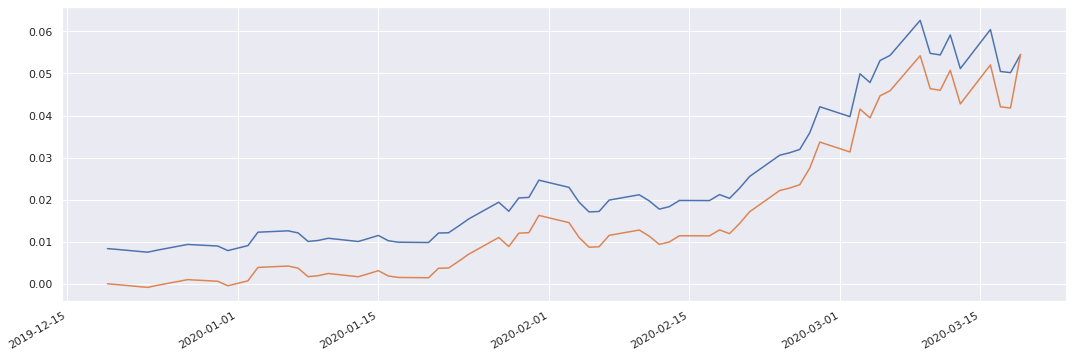
You can then comparatively plot the histories of both swaptions:
s.history().plot()
s_fp.history().plot()
Cash vs physical settlement#
The swaption group determines whether the swaption is cash or swap settled. As mentioned above, all swaptions—except for EUR and GBP—are swap settled. Resetting the cash_settled field of the swaption group resets this behaviour.
It is possible to cash settle EUR swaptions (or any other currency) by setting the cash_settled_with_swap_rate input of the Swaption class to True.
Metrics#
The main valuation function is swaption_metrics which computes various metrics for required dates. By default, all history dates are used and if fields are omitted, all current possible metrics—'NPV', 'Delta', 'Gamma', 'Theta', 'Vega', 'ParRate' and 'ImpliedVolatility'—are computed.
Input:
s.swaption_metrics()
Output:
		NPV	        Delta		Gamma		Theta		Vega		ImpliedVolatility ParRate       ATMVol
2019-12-19	0.008366	-3.026291	6.092862e+02	-2.904796e-05	9.005980e-01	0.005929	0.017177	0.006016
2019-12-20	0.008170	-2.998189	6.166100e+02	-2.932279e-05	9.000538e-01	0.005920	0.017229	0.006005
2019-12-23	0.007511	-2.876380	6.354629e+02	-3.059697e-05	9.015133e-01	0.005952	0.017431	0.006024
2019-12-24	0.008018	-2.988126	6.257035e+02	-3.037099e-05	8.813905e-01	0.005979	0.017257	0.006062
2019-12-27	0.009359	-3.281607	5.970830e+02	-2.891643e-05	8.119626e-01	0.005980	0.016804	0.006083
...	...	...	...	...	...	...	...	...
2020-03-12	0.059147	-4.967608	1.571852e-03	4.025946e-07	5.042917e-07	0.016729	0.006270	0.014416
2020-03-13	0.051148	-4.953404	1.151454e-04	7.207563e-07	2.689915e-08	0.014211	0.007851	0.012426
2020-03-16	0.060423	-4.969253	4.364755e-21	2.555868e-07	4.616290e-25	0.012868	0.006017	0.009700
2020-03-17	0.050462	-4.950216	4.179410e-28	2.288431e-07	2.650554e-32	0.011574	0.007983	0.009050
2020-03-18	0.050184	-4.954347	2.677865e-42	-5.018369e-02	9.860266e-47	0.013440	0.008047	0.011479
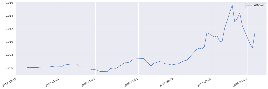
To plot the time series for a particular metric by specifying a field:
s.swaption_metrics(fields = 'ATMVol').plot()
Greeks#
Vega is sensitivity to a 1bp change in volatility.
Delta is sensitivity to a 1bp change in swap rate.
Gamma is change in delta per 1bp change in swap rate.
Input:
s.pnl_explain()
Output:
		Delta			Gamma	Vega	Theta	Actual	Explained	Residual	Explained pct	Residual pct
2019-12-20	-0.000157	1.649058e-06	-8.020299e-06	-2.904796e-05	-0.000195	-0.000193	-0.000002	98.7	1.3
2019-12-23	-0.000606	2.517119e-05	2.887594e-05	-8.796836e-05	-0.000659	-0.000640	-0.000019	97.1	2.9
2019-12-24	0.000500	1.919946e-05	2.400588e-05	-3.059697e-05	0.000506	0.000513	-0.000006	101.2	-1.2
2019-12-27	0.001352	1.281184e-04	1.477844e-06	-9.111298e-05	0.001341	0.001391	-0.000049	103.7	-3.7
2019-12-30	-0.000417	9.634462e-06	1.179894e-04	-8.674930e-05	-0.000384	-0.000376	-0.000008	97.8	2.2
...	...	...	...	...	...	...	...	...	...
2020-03-13	-0.007852	3.927438e-09	-1.269563e-09	4.025946e-07	-0.007999	-0.007852	-0.000147	98.2	1.8
2020-03-16	0.009082	3.870609e-10	-3.613826e-11	2.162269e-06	0.009274	0.009084	0.000191	97.9	2.1
2020-03-17	-0.009767	1.686088e-26	-5.972506e-28	2.555868e-07	-0.009961	-0.009767	-0.000194	98.0	2.0
2020-03-18	-0.000320	1.746410e-36	4.945335e-35	2.288431e-07	-0.000278	-0.000320	0.000042	115.0	-15.0
2020-03-19	0.004168	1.895655e-48	0.000000e+00	-5.018369e-02	0.004314	-0.046015	0.050330	-1066.6	1166.6
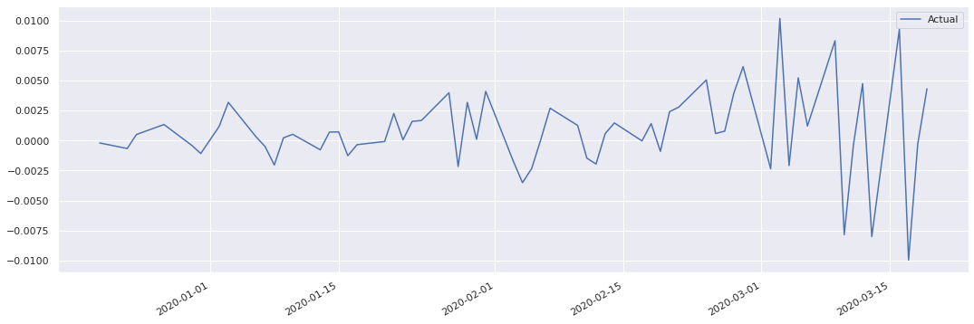
To plot the time series for a particular value by specifying a field:
s.pnl_explain(fields="Actual").plot()
Building blocks#
Like with options, the SigTech framework supports basic functionality for rolling swaptions, straddle and strangle with sig.RollingSwaption, sig.SwaptionStraddle and sig.SwaptionStrangle. The parameters are the same as those used in the corresponding option strategies, with the only differences being that swaption strategies require an underlying swap_tenor and don’t require a group_name—which can be obtained by default from currency.
The functionality for the option strategies—option_position_greeks, portfolio_greeks, output_option_position_diagnostics—is largely the same.
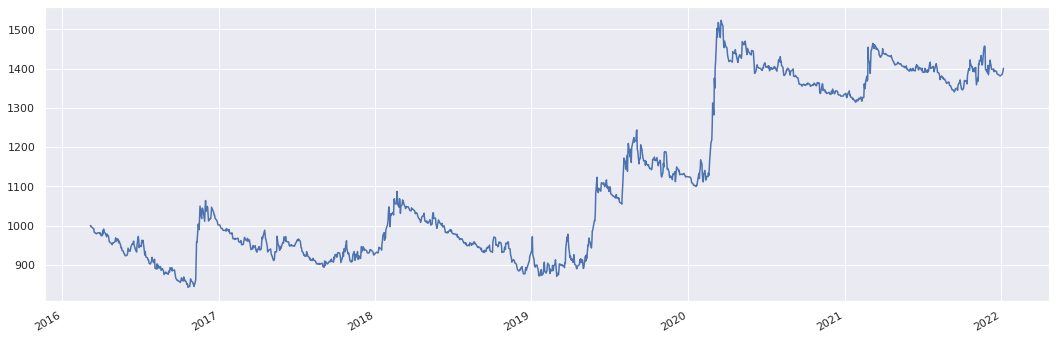
RollingSwaption#
from sigtech.framework.strategies.rolling_swaption_baskets import RollingSwaption
usd_rolling_swaption  = RollingSwaption(
    start_date=dtm.date(2016, 3, 5),
    maturity="6M",
    currency="USD",
    group_name=sig.SwaptionGroup.get_group("USD").name,
    rolling_frequencies=["3M"],
    swaption_type="Payer",
    target_type="Fixed",
    target_quantity=1000,
    include_trading_costs=False,
    total_return=False,
    swap_tenor="30Y"
)
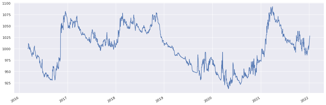
usd_rolling_swaption.history().plot()
<matplotlib.axes._subplots.AxesSubplot at 0x7f2b02a34390>
Input:
usd_rolling_swaption.plot.timeline()
Output:
VBox(children=(HBox(children=(Button(button_style='primary', description='Refresh', layout=Layout(max_width='9…
Input:
usd_rolling_swaption.option_position_greeks(dtm.datetime(2018,1,5),field = "Vega")
Output:
{'USD SWAPTION GROUP': 5544.3174445353425}
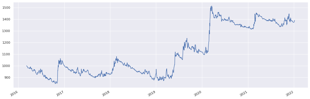
sig.SwaptionStraddle#
usd_rolling_straddle = sig.SwaptionStraddle(
    start_date=dtm.date(2016, 3, 5),
    maturity="6M",
    currency="USD",
    group_name=sig.SwaptionGroup.get_group("USD").name,
    rolling_frequencies=["3M"],
    strike_type="SPOT",
    close_out_at_roll=True,
    include_trading_costs=False,
    total_return=False,
    target_type="Fixed",
    target_quantity=10000,
    swap_tenor="5Y"
)
usd_rolling_straddle.history().plot()
Input:
usd_rolling_straddle.portfolio_greeks()
Output:
NPV	Delta	Gamma	Vega	ImpliedVolatility
USD 54F346FF SS STRATEGY	USD SWAPTION GROUP	USD SWAPTION GROUP	USD SWAPTION GROUP	USD SWAPTION GROUP
2016-03-07	0.000000	0.000000	0.000000e+00	0.000000	NaN
2016-03-08	1000.000000	0.000000	0.000000e+00	0.000000	NaN
2016-03-09	1000.000000	-5577.225450	6.593613e+06	27210.642946	0.008231
2016-03-10	996.544960	-3250.792135	6.683914e+06	27300.181024	0.008191
2016-03-11	996.227388	720.943430	6.671492e+06	27271.548621	0.008243
...	...	...	...	...	...
2021-12-30	1382.706878	4019.385157	7.542653e+06	25354.067507	0.007716
2022-01-04	1381.884868	1145.094125	7.619412e+06	25423.285774	0.007708
2022-01-05	1385.361424	8589.316047	7.427516e+06	24364.490809	0.007826
2022-01-06	1389.110628	14523.718855	7.235895e+06	23058.831646	0.007652
2022-01-07	1393.834792	17412.781679	7.030082e+06	22160.267776	0.007620
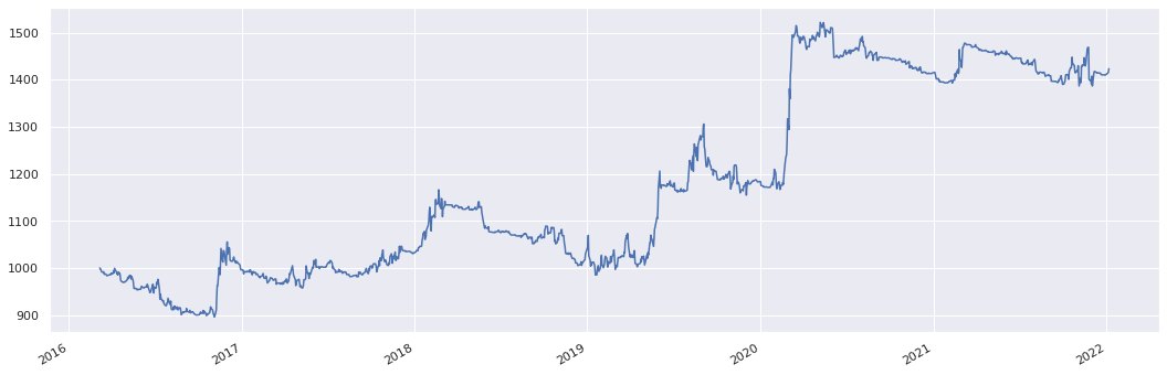
sig.SwaptionStrangle#
usd_rolling_strangle = sig.SwaptionStrangle(
    start_date=dtm.date(2016, 3, 5),
    maturity="6M",
    currency="USD",
    group_name=sig.SwaptionGroup.get_group("USD").name,
    rolling_frequencies=["3M"],
    receiver_strike="ATM+10bp",
    payer_strike="ATM-10bp",
    close_out_at_roll=True,
    include_trading_costs=False,
    total_return=False,
    target_type="Fixed",
    target_quantity= 10000,
    swap_tenor="5Y"
)
usd_rolling_strangle.history().plot()
Delta hedging#
Like with strategies inheriting from the rolling_options_basket class, all swaption strategies, including SwaptionStraddle and SwaptionStrangle, can use the DeltaHedgingStrategy as an input with hedging_instrument_type set to 'UNDERLYING'.
If include_option_strategy is set to False it will produce an equivalent strategy obtained by trading the delta amounts of the underlying swap.
If include_option_strategy is set to True it will produce a delta hedge of the original strategy.
sig.DeltaHedgingStrategy?
usd_strangle_dh = sig.DeltaHedgingStrategy(
    currency = "USD",
    start_date = dtm.date(2016,3,5),
    option_strategy_name = usd_rolling_strangle.name,
    hedging_instrument_type = "UNDERLYING",
    include_option_strategy = False,
    rebalance_hedge_on_roll= False
    # you can choose for hedge adjustments to occur only on dates when the options are rolled
)
usd_strangle_dh.history().plot()
Input:
usd_strangle_dh.plot.portfolio_table()
Output:
Collapse All Expand Strategies Partial Expand Expand All
None Positions Cash Orders
MENU
FILTER:
None
Position Type
Value (local)
Value
Units
Valuation
Exp. Weight
Weight
Execution Time
Input:
usd_strangle_dh.plot.timeline()
Output:
VBox(children=(HBox(children=(Button(button_style='primary', description='Refresh', layout=Layout(max_width='9…
Additional building blocks#
from sigtech.framework.strategies.rolling_swaption_baskets import *
The Dynamic Swaptions Strategy trades a custom basket of swaptions.
DynamicSwaptionsStrategy?
The Dynamic Multi Swaptions Strategy trades a basket of swaptions from multiple groups.
DynamicMultiSwaptionsStrategy?
Transaction costs#
A vega-based transaction cost is used, with scaling parameters defined in the SWAPTION_VOL_TCOST dictionary of sigtech/framework/transaction_cost/constants.py. There is a default scale of 5 vega basis points, and a currency specific scale of 2bp for USD and EUR (i.e. t-cost is vega*0.0002).
Input:
sig.TradePricer.get_tc_model(s.name)
Output:
{'name': 'vega_based_positive',
 'parameters': {'default': 0.05, 'USD': 0.02, 'EUR': 0.02},
 'source': 'Swaption',
 'info': 'Transaction cost model: vega_based_positive\nModel docstring:  Price adjusted by transaction cost based on a multiple of vega, limited by zero to avoid over-adjustment and negative prices.  '}