Data Analysis

Primer on CLS data analysis.

Introduction

CLS operates the largest multi-currency cash settlement system.

CLS Market Data is a comprehensive suite of FX alternative data products designed to provide quality insight for financial efficiency, visibility and control.

These data sets can be accessed and analysed in the SigTech platform.

In this primer we give a few examples of analysing the data and creating simple strategies that use a signal generated from this data.

The output is generated from the provided code examples. These examples can be fully customised or extended.

A notebook containing all the code used in this page can be accessed in the research environment: Example notebooks.

Environment

This section will import relevant internal and external libraries, as well as setting up the platform environment. For further information in regards to setting up the environment, see Environment setup.

import sigtech.framework as sig
from sigtech.framework.analytics.cls_data import ClsData, CLS_DATASETS, CLS_FREQ, CLS_INSTRUMENTS, CLS_PUBLICATION_FREQ, \
    resample_reduced, remove_weekends, CLS_CCY_CROSSES
from sigtech.framework.infra.objects.dtypes import AnyType

import datetime as dtm
import numpy as np
import pandas as pd
import matplotlib.pyplot as plt
import pytz
import seaborn as sns

sns.set(rc={'figure.figsize': (18, 6)})

if not sig.config.is_initialised():
    env = sig.config.init()

Here we set the source of FX data to CLS, this causes the CLS pricing data to be used in simulations.

A CLS data class (ClsData) is then created. This instance provides access to the various data sets and parameters.

We initialize the class with a list of default currencies to retrieve data for when no specific currency cross is requested.

For demonstration purposes we limit this to a subset of available currencies but the full list is given by CLS_CCY_CROSSES.

# Set fx source to use CLS data
env[sig.config.CUSTOM_DATA_SOURCE_CONFIG] = [
    ('[A-Z]{6} CURNCY', 'CLS'),
]

EXCLUDED_CCYS = {'USDILS', 'EURHUF', 'EURDKK', 'USDHUF', 'USDDKK', 'USDKRW'}
ccys_included = sorted(set(CLS_CCY_CROSSES) - EXCLUDED_CCYS)
cls_data = ClsData(ccys_included[:3])

CLS Data Examples

Liquidity times

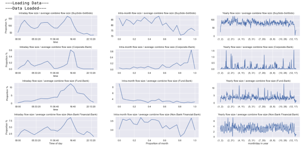
The hourly trade flows can be normalised per currency cross and grouped to give an estimate for the proportion of volume traded by the different counter parties. These proportions are plotted below on an hourly, monthly and yearly period. This shows the time windows with highest liquidity. This is combined for the crosses but could be split out for individual currencies.

A few minutes are required to pull in the required data for the first run.

Python

# Load data
print('---Loading Data---')
flow_direction_base, flow_size_base = cls_data.spot_hourly_flow_df(cross_list=cls_data.crosses)
print('---Data Loaded---')


def daysinmonth(year, month):
    """ Helper method to calculate. number of days in a month. """
    dt = dtm.date(year, month, 1)
    if month == 12:
        next_dt = dtm.date(year + 1, 1, 1)
    else:
        next_dt = dtm.date(year, month + 1, 1)
    return (next_dt - dt).days


fig = plt.figure(figsize=(20, 9))
scaled_vol_flow = 100 * (flow_size_base.stack(2) / flow_size_base.sum(axis=1, level=(0, 1)).mean())[
    cls_data.half_pairs].unstack(1).sort_index(axis=0)

for i in range(4):
    df = scaled_vol_flow.groupby(lambda x: x.time).mean().mean(axis=1, level=2)
    ax = plt.subplot2grid((4, 3), (i, 0), fig=fig)
    df.iloc[:, i].plot(ax=ax, title='Intraday flow size / average combine flow size ({})'.format(df.columns[i]));
    ax.set_ylabel('Proportion %')
ax.set_xlabel('Time of day')

# resample to daily points that existed in original data
daily_scaled_vol_flow = resample_reduced(scaled_vol_flow, rule='1D', method='mean')
for i in range(4):
    df = (
        daily_scaled_vol_flow.groupby(lambda x: (1 / 21) * int(21 * x.day / daysinmonth(x.year, x.month))).mean()).mean(
        axis=1, level=2)
    ax = plt.subplot2grid((4, 3), (i, 1), fig=fig)
    df.iloc[:, i].plot(ax=ax, title='Intra-month flow size / average combine flow size ({})'.format(df.columns[i]));
ax.set_xlabel('Proportion of month')

for i in range(4):
    df = (daily_scaled_vol_flow.groupby(lambda x: (x.month, x.day)).mean()).mean(axis=1, level=2)
    ax = plt.subplot2grid((4, 3), (i, 2), fig=fig)
    df.iloc[:, i].plot(ax=ax, title='Yearly flow size / average combine flow size ({})'.format(df.columns[i]));
ax.set_xlabel('month/day in year')
plt.tight_layout()

Output

The relationship between hourly trade activity on spot market moves

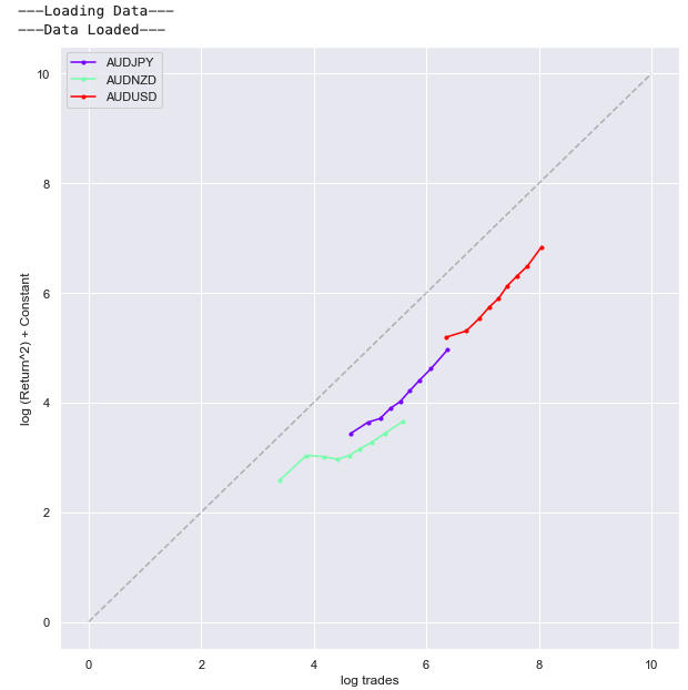
By grouping the price moves in buckets of different trade counts we can look at how the magnitude of price moves are related to the number of trades. The relationship between the trade counts and the squared hourly returns can be observed in the chart below. Each point represents a decile bucket. This information could be used to calibrate the persistent price impact in transaction cost models or use volume forecasts to predict volatility.

Python

print('---Loading Data---')
trades = cls_data.data(cls_data.SPOT_VOLUME_HOURLY_DAILY)
prices = cls_data.spot_prices_df(cross_list=cls_data.crosses, add_inverse=False)
print('---Data Loaded---')


def digitize_ts(ts, bins=10):
    bins = np.linspace(ts.min(), ts.max() + 1e-9, bins + 1)
    return pd.Series(index=ts.index, data=[bins[i] for i in np.digitize(ts, bins=bins)])


def digitize_df(df, bins=10, columns=None):
    if columns is None:
        columns = df.columns
    dfc = df.copy()
    for col in columns:
        dfc[col] = digitize_ts(df[col], bins=bins)
    return dfc


cross_trades_vs_rt = []
for cross in cls_data.crosses:
    df = pd.concat({'rt': prices[(cross[:3], cross[3:])].pct_change(),
                    'trades': trades[cross]['trades']}, axis=1).dropna()

    # A constant is calculated to shift the different currency crosses based on a measure of their liquidity.
    constant = - np.log(df['rt'].var() / df['trades'].mean())

    df['rt^2'] = df['rt'] ** 2
    df = df[df['trades'].abs() > 0]

    # Evaluate digitized percentiles
    digitized_percentile_df = digitize_df(df.rank(pct=True, method='first'), bins=10, columns=['rt', 'trades', 'rt^2'])

    # Group deciles
    grouped_percentiles = digitized_percentile_df.groupby('trades').mean()['rt^2']

    # invert percentiles to values for display
    grouped_percentiles.index = np.interp(grouped_percentiles.index,
                                          df['trades'].rank(pct=True, method='first').sort_values(),
                                          np.log(df['trades'].sort_values()))
    grouped_percentiles.iloc[:] = np.interp(grouped_percentiles.values,
                                            df['rt^2'].rank(pct=True, method='first').sort_values(),
                                            np.log(df['rt^2'].sort_values()))
    grouped_percentiles.name = cross

    cross_trades_vs_rt.append(grouped_percentiles.iloc[0:9] + constant)

colors = plt.cm.rainbow(np.linspace(0, 1, len(cross_trades_vs_rt)))

for _s, _c in zip(cross_trades_vs_rt, colors):
    ax = _s.plot(legend=True, figsize=(10, 10), style='.-', c=_c)

ax.plot((0, 10), (0, 10), color='k', linestyle='--', alpha=0.25)
ax.set_xlabel('log trades')
ax.set_ylabel('log (Return^2) + Constant');

Output

Corporate flow correlations

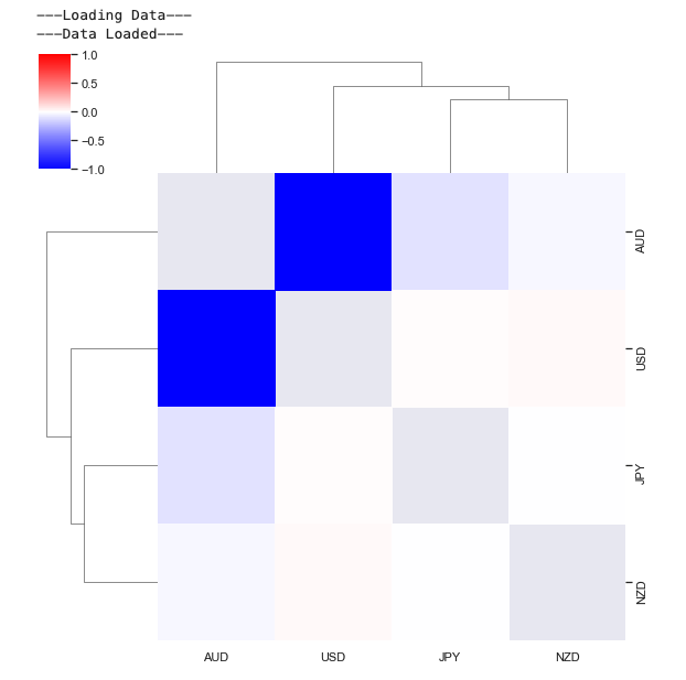
The correlations between USD corporate-bank flows are calculated below and shown in a hierarchical correlation plot. First we amalgamate the currency cross flows to obtain total flow into and out of each currency. We can then consider the correlations between these flows. This is done below on 48-hour intervals for the corporate flow data.

This indicates groupings of currencies and shows a strong negative correlation between USD and EUR flow.

Python

print('---Loading Data---')
flow_direction_usd, flow_size_usd = cls_data.spot_hourly_flow_df(cross_list=cls_data.crosses, convert_to_ccy='USD')
print('---Data Loaded---')

flow_data = flow_direction_usd.sum(axis=1, level=(2, 0))['Corporate-Bank']
sns.clustermap(resample_reduced(flow_data, rule='48H', method='mean').corr(),
               mask=np.identity(len(flow_data.columns)),
               figsize=(8, 8), vmin=-1, vmax=1, cmap='bwr');

Output

Autocorrelations

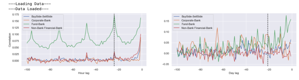
Autocorrelations can be observed in the flow data. Plots of Spearman autocorrelations are shown below on hourly and daily timeframes. For the hourly analysis, all of the counter party flows exhibit autocorrelation, but this is focused at the daily lagged points. In the case of daily autocorrelations they are much stronger for corporate flows with monthly lags.

Python

print('---Loading Data---')
flow_direction_usd, flow_size_usd = cls_data.spot_hourly_flow_df(cross_list=cls_data.crosses, convert_to_ccy='USD')
print('---Data Loaded---')


def calc_autocorr_plot(x, y=None, lags=10):
    """ Method to return autocorrelations. """
    if y is None:
        y = x
    res = [pd.concat([x, y.shift(l)], axis=1).dropna().corr().iloc[0, 1] for l in range(-lags, 1)]
    return pd.Series(index=range(-lags, 1), data=res)


# Percentiles used for Spearman autocorrelations
combined_ccy_flow = flow_direction_usd.sum(axis=1, level=(0, 2))
cpty_combined_ccy_flow = combined_ccy_flow.rank(pct=True).stack(0).reorder_levels((1, 0)).sort_index()

daily_combined_ccy_flow = resample_reduced(combined_ccy_flow, rule='1B', base=22, method='sum')
cpty_daily_combined_ccy_flow = daily_combined_ccy_flow.rank(pct=True).stack(0).reorder_levels((1, 0)).sort_index()

# Calculate autocorrelations
hourly_autocorr = {}
daily_autocorr = {}

for col in cpty_combined_ccy_flow.columns:
    hourly_autocorr[col] = calc_autocorr_plot(cpty_combined_ccy_flow.loc[:, col], lags=100).iloc[:-1]

for col in cpty_daily_combined_ccy_flow.columns:
    daily_autocorr[col] = calc_autocorr_plot(cpty_daily_combined_ccy_flow.loc[:, col], lags=100).iloc[:-1]

# Plot Autocorrelations
fig = plt.figure(figsize=(20, 4))
ax = plt.subplot2grid((1, 2), (0, 0), fig=fig)
pd.DataFrame(hourly_autocorr).plot(ax=ax)
ax.set_ylabel('Correlation')
ax.set_xlabel('Hour lag')
ax.axvline(-24, color='k', linestyle='--')

ax = plt.subplot2grid((1, 2), (0, 1), fig=fig)
pd.DataFrame(daily_autocorr).plot(ax=ax)
ax.set_xlabel('Day lag')
ax.axvline(-21, color='k', linestyle='--');

Output

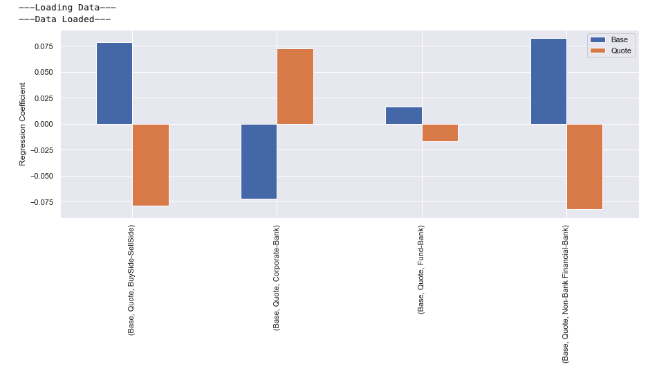
Directional logistic regression

A logistic regression on the direction of the movement can be performed with the normalised logarithm of flows as the inputs. The coefficients then reveal the relationship between the flows against the preference of direction. Interestingly, the corporate flow has a negative relationship suggesting that the larger the corporate flow in to a currency the greater the chance the value will decrease.

Python

print('---Loading Data---')
flow_direction_usd, flow_size_usd = cls_data.spot_hourly_flow_df(cross_list=cls_data.crosses, convert_to_ccy='USD')
prices_df = cls_data.spot_prices_df(cross_list=cls_data.crosses, add_inverse=True)
print('---Data Loaded---')


def slog(x):
    return np.sign(x) * np.log(1 + np.abs(x))


from sklearn.linear_model import LogisticRegression

lr = LogisticRegression(C=1, fit_intercept=True)

combined_ccy_flow = flow_direction_usd.sum(axis=1, level=(0, 2))
combined_ccy_size = flow_size_usd.sum(axis=1, level=(0, 2))

stackf = []
stackp = []
for pair in cls_data.pairs:
    am_flow = combined_ccy_flow[[pair[0], pair[1]]]

    am_flow = slog(am_flow)
    am_flow = (am_flow - am_flow.mean())
    am_flow /= am_flow.abs().max()

    prices = np.log(prices_df.ffill()).diff()[[pair]].dropna()
    prices = (prices - prices.mean()) > 0

    idx = am_flow.index.intersection(prices.index)
    f, p = (am_flow.reindex(idx)), (prices.reindex(idx))

    stackf.append(f.iloc[:].values)
    stackp.append(p.iloc[:].values)

stackf = np.vstack(stackf)
stackp = np.vstack(stackp)
lr.fit(stackf[:], stackp[:])

df = pd.DataFrame(index=pd.MultiIndex.from_tuples([('Base', 'Quote')]),
                  columns=pd.MultiIndex.from_tuples(
                      [(x[0].replace(cls_data.pairs[-1][0], 'Base').replace(cls_data.pairs[-1][1], 'Quote'), x[1]) for x
                       in am_flow.columns]),
                  data=np.atleast_2d(lr.coef_)).stack()

ax = df.plot(kind='bar', figsize=(15, 5));
ax.set_ylabel('Regression Coefficient');

Output

Forward trades

The CLS forward data contains information on the volume of forwards traded each hour and their corresponding delivery dates. As an example of the information present in this data, the plot below shows the daily traded volumes of forwards covering different windows in the future. Steps, indicating popular delivery periods, can be observed at 3, 6, 9 and 12 months and a roll down to the quarterly roll dates.

Python

print('---Loading Data---')
daily_fwd_volume = cls_data.data(cls_data.FWD_VOLUME_DAILY_DAILY, cross_list=['EURUSD'])
print('---Data Loaded---')

fwd_grid = pd.DataFrame({x[0]: pd.Series(
    index=list(range(min(500, len(pd.date_range(x[1]['window_end'].date(), x[0][1].date()))))), data=x[1]['volume'])
    for x in daily_fwd_volume['EURUSD'].iterrows() if x[1]['volume'] > 0}).fillna(0).T.groupby(
    level=0).sum()
fwd_grid.index = fwd_grid.index.date

fig = plt.figure(figsize=(20, 6))
sns.heatmap(np.log(1 + fwd_grid.T.iloc[500:0:-1, :]));
plt.gca().set_xlabel('Trade Date')
plt.gca().set_ylabel('Days in to the future')
plt.gca().set_title('Logarithm of span for total forward volume traded');

Output

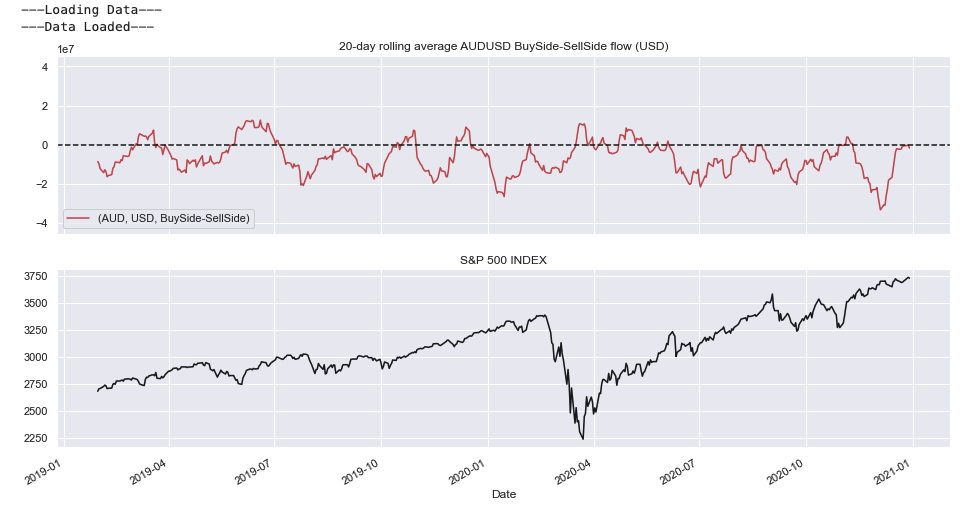
Flow vs Equity Comparison

In the interactive visualisation below we track the average 20-day flow versus US Equity market during 2020.

Large flows are observed to USD from EUR during the onset of the corona virus epidemic.

To enable the interactive visualisation uncomment the interact decorator and remove the plot.

Python

print('---Loading Data---')
flow_direction_usd, flow_size_usd = cls_data.spot_hourly_flow_df(cross_list=cls_data.ccy_crosses, convert_to_ccy='USD')
print('---Data Loaded---')

flow_data = flow_direction_usd.dropna().loc[dtm.date(2019, 1, 1):dtm.date(2021, 1, 1)]
flow_data = flow_data.rolling(window=20 * 24).mean().dropna()
flow_data = resample_reduced(flow_data, rule='1D', method='last')

maxv = (np.abs(flow_data).max().max())
ccy_list = set(flow_data.columns.get_level_values(level=0))
cpty_list = sorted(set(flow_data.columns.get_level_values(level=2)))

# Load S&P 500 INDEX data
equity_ts = sig.obj.get('SPX INDEX').history().reindex(flow_data.index, method='ffill')

import ipywidgets as ipy


# @ipy.interact(base=ccy_list, quote=ccy_list, cptys=cpty_list)
def plot_comparison(base='AUD', quote='USD', cptys='BuySide-SellSide'):
    fig = plt.figure(figsize=(16, 8))
    ax = plt.subplot2grid((2, 1), (0, 0))

    if base != quote:
        ax = flow_data[(base, quote, cptys)].plot(color='r', legend=True, ax=ax, ylim=(-maxv, maxv))
    ax.legend(loc="lower left")
    ax.axhline(0, color='k', linestyle='--')

    ax.set_title('20-day rolling average {} {} flow (USD)'.format(base + quote, cptys))
    ax = plt.subplot2grid((2, 1), (1, 0), sharex=ax)
    equity_ts.plot(ax=ax, legend=False, color='k')
    ax.set_title('S&P 500 INDEX')
    ax.set_xlabel('Date')
    plt.show();


plot_comparison()

Output

Intraday strategy simulation

Traditional trading strategies such a FX carry, value and momentum have severely underperformed over the past 10 years. By the use of CLS flow data a simple trading strategy can be constructed.

The SigTech platform can run systematic trading simulations. Here two strategies are simulated that trade FX spot based on signals generated from CLS data.

For further information regarding the strategy API please see the SigTech example notebooks.

Signal based on flow direction

Here we define a strategy which trades one spot FX cross in the same direction as the 'BuySide-SellSide' flow was 24 hours prior. This makes use of the autocorrelation observed in the flows.

class SimpleFXSpotStrategy(sig.Strategy):
    
    # Specify Strategy parameters
    ccy = AnyType(required=True)
    
    def __init__(self):
        super().__init__()
        
        # retrieve CLS flow data for cross.
        flow_direction_base, flow_size_base = cls_data.spot_hourly_flow_df(cross_list=[self.ccy + self.currency], 
                                                                           intraday='matched')
        
        # Calculate signal
        signal = np.sign(flow_direction_base[(self.ccy, self.currency, 'BuySide-SellSide')])
        signal.index = [pytz.utc.localize(dt) for dt in signal.index]
        self.signal = remove_weekends(signal).rolling(window=2).mean()

    def strategy_initialization(self, dt):
        
        # setup strategy hourly rebalancing.
        for rdt in self.signal.loc[self.calculation_start_dt():self.calculation_end_dt()].index:
            if rdt > dt:
                self.add_method(rdt, self.rebalance, use_trading_manager_calendar=False)
                
    def rebalance(self, dt):
        
        # Determine strategies cash holdings and value.
        current_base = self.positions.get_cash_value(dt, '{} CASH'.format(self.ccy))
        current_ccy = self.positions.get_cash_value(dt, '{} CASH'.format(self.currency))
        value = self.positions.valuation(dt, self.ccy)
        
        # Get signal value to rebalance to.
        direction = (self.signal.asof(dt - dtm.timedelta(hours=22)))
        
        # Perform an fx spot trade.
        self.add_fx_spot_trade(dt, self.currency, self.ccy, value * direction - current_base, execution_dt=dt, use_trading_manager_calendar=False)
        
    def size_dt_from_decision_dt(self, decision_dt):
        return decision_dt - dtm.timedelta(hours=1)

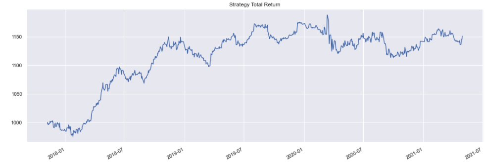
The strategy is now initialised and run for USDJPY. Here we exclude transaction costs to give a cleaner measure of the signals predictive power.

Python

simple_strategy = SimpleFXSpotStrategy(currency='USD', ccy='EUR', start_date=dtm.date(2017, 11, 6),
                                       include_trading_costs=False)
strategy_ts = simple_strategy.history()

strategy_ts.plot(title='Strategy Total Return');

Output

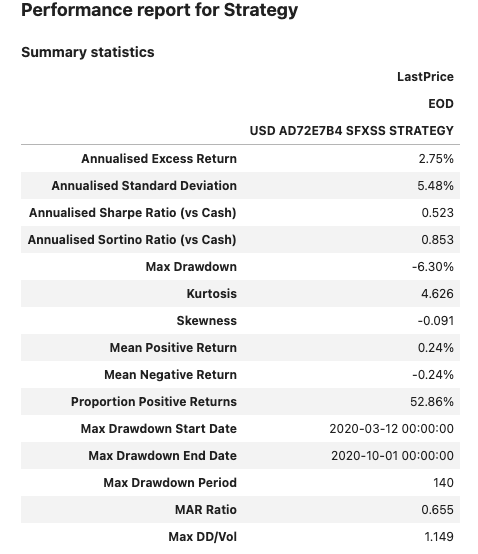
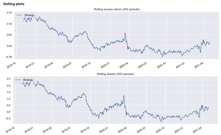
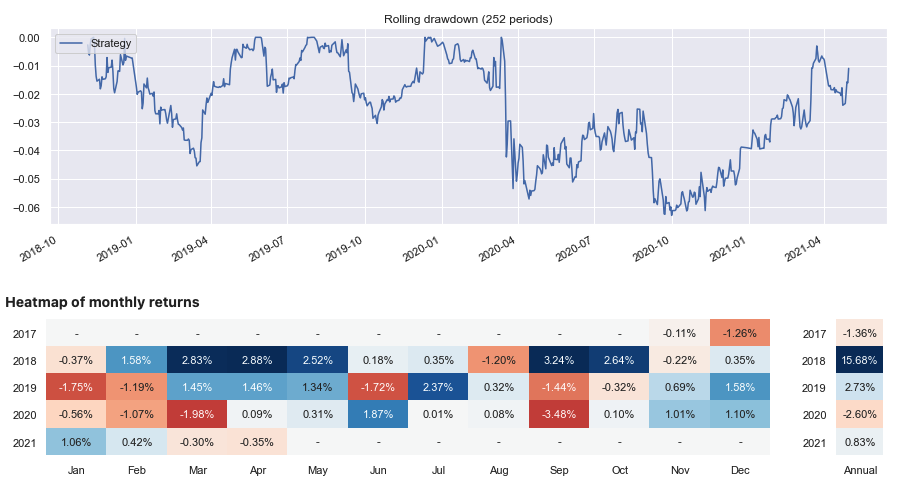
A performance report for this strategy can then be generated.

Python

sig.PerformanceReport(strategy_ts, cash=sig.CashIndex.from_currency('USD')).report()

Output

Signal based on weighted prices

The following strategy combines the volume from the CLS flow data with the pricing data to give a 24 hour VWAP. A signal is then calculated which assumes that the price will move towards this level.

def vol_weight(data, weights, window):
    sum_prod = ((weights).multiply(data, axis=0)).dropna()
    sum_vol = (weights.reindex(sum_prod.index)).rolling(window=window).sum()
    sum_prod = sum_prod.rolling(window=window).sum()
    return sum_prod.divide(sum_vol, axis=0).dropna()

class VWAPStrategy(sig.Strategy):
    # Specify Strategy parameters
    ccy = AnyType(required=True)
    cpty_group = AnyType(default=None)
    
    def __init__(self):
        super().__init__()
        self.signal = self.calculate_signal()
    
    def calculate_signal(self):
        cross = self.ccy + self.currency
        
        prices = cls_data.data(cls_data.SPOT_PRICE_5MIN_DAILY, cross_list=[cross])[cross]['twap'].ffill().dropna()
        _ , hourly_sizes = cls_data.spot_hourly_flow_df([cross], intraday='matched')
        hourly_sizes = hourly_sizes[(self.ccy, self.currency, self.cpty_group)]
        hourly_prices = resample_reduced(prices, rule='1H', method='last')
        
        rolling_hourly_vwap = vol_weight(hourly_prices, hourly_sizes, window=24)
        signal = rolling_hourly_vwap - hourly_prices
        signal = signal.divide(signal.rolling(window=24*10).std()).dropna()
        signal.index = [pytz.utc.localize(dt) for dt in signal.index]
        return remove_weekends(signal)
                             
    def strategy_initialization(self, dt):
        
        # setup strategy hourly rebalancing.
        for rdt in self.signal.loc[self.calculation_start_dt():self.calculation_end_dt()].index:
            if rdt > dt:
                self.add_method(rdt, self.rebalance, use_trading_manager_calendar=False)
                
    def rebalance(self, dt):
        
        # Determine strategies cash holdings and value.
        current_base = self.positions.get_cash_value(dt, '{} CASH'.format(self.ccy))
        current_ccy = self.positions.get_cash_value(dt, '{} CASH'.format(self.currency))
        value = self.positions.valuation(dt, self.ccy)
        
        # Get signal value to rebalance to. A lag of 1 hour is applied.
        direction = (self.signal.asof(dt - dtm.timedelta(hours=1)))
        
        # Clip signal
        direction = 0.5 * min(max(direction, -2), 2)
        
        # Perform an fx spot trade.
        self.add_fx_spot_trade(dt, self.currency, self.ccy, value * direction - current_base, execution_dt=dt, use_trading_manager_calendar=False)
        
    def size_dt_from_decision_dt(self, decision_dt):
        return decision_dt - dtm.timedelta(hours=1)

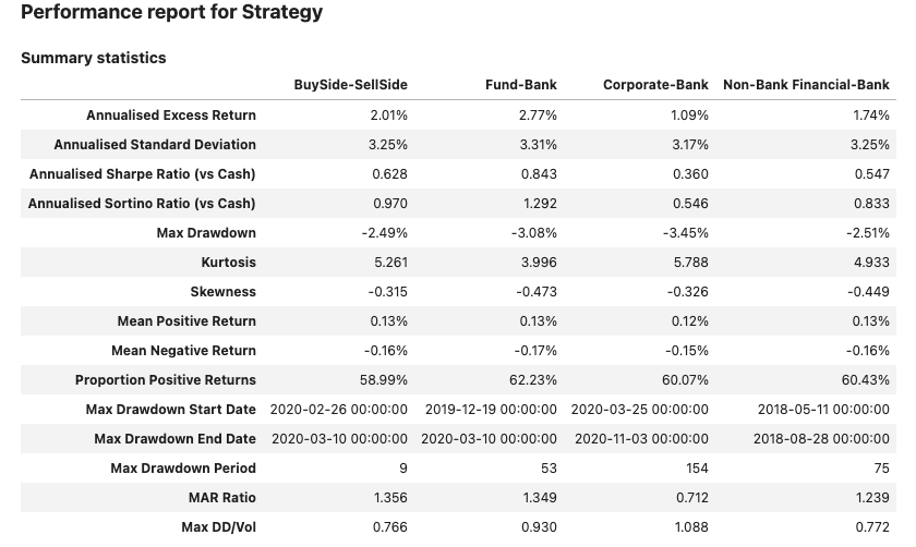
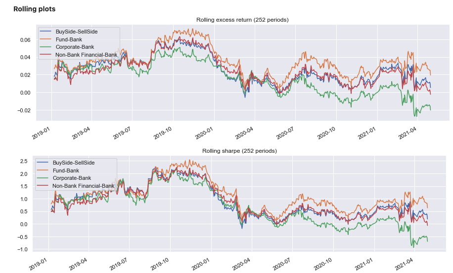
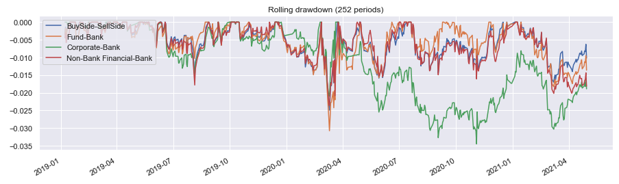
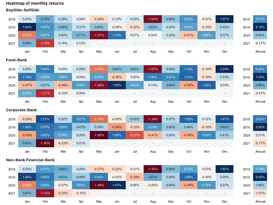
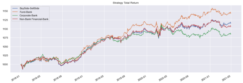
This strategy is run below for the 'EURUSD' cross and each counter party grouping of flow. A benefit can be observed for using the prices weighted by fund trade volumes. Here we exclude transaction costs to give a cleaner measure of the signals predictive power.

Python

ax = None
strategy_ts_dict = {}
for cpty_group in ('BuySide-SellSide', 'Fund-Bank', 'Corporate-Bank', 'Non-Bank Financial-Bank'):
    simple_strategy = VWAPStrategy(currency='USD',
                                   ccy='EUR',
                                   cpty_group=cpty_group,
                                   start_date=dtm.date(2018, 1, 4),
                                   include_trading_costs=False)
    strategy_ts = simple_strategy.history()
    strategy_ts_dict[cpty_group] = strategy_ts

    ax = strategy_ts.plot(label=cpty_group, ax=ax, legend=True)
    
ax.set_title('Strategy Total Return');

Output

Python

sig.PerformanceReport(pd.DataFrame(strategy_ts_dict), cash=sig.CashIndex.from_currency('USD')).report()

Output