Pandas introduction#
This section introduces some basic functionality of the Python pandas data analysis package, and aims to ensure that all users are able to rapidly backtest realistic strategies.
Note: the pandas library underlies parts of the SigTech Framework and is widely used in example notebooks.
Sections#
Importing modules#
Import the datetime module with the alias dtm. This module is used in defining dates, times, and more.
It is also useful for creating schedules and performing analysis of data indexed by dates and timestamps.
import datetime as dtm
Import the pandas data analysis module under the alias pd:
import pandas as pd
Import the numpy numerical computing module under the alias np:
import numpy as np
Import the matplotlib.pyplot library for plotting under the alias plt:
import matplotlib.pyplot as plt
Import the plotting library seaborn under the alias sns. Set the default figure size for all plots within the notebook:
import seaborn as sns
sns.set(rc={'figure.figsize': (18, 6)})
Import and initialise the SigTech Framework:
import sigtech.framework as sig
end_date = dtm.date(2021, 12, 31)
sig.init(env_date=end_date)
Pandas objects#
The SigTech platform is object-oriented in design: every asset is modelled as a different object with its own attributes, methods and attached datasets.
Fetch a SingleStock object:
stock = sig.obj.get('1000045.SINGLE_STOCK.TRADABLE')
Pandas series objects#
A historical time series of an asset’s value can be obtained by calling the history method on that asset. This returns a pandas Series(pd.Series) object, whose values are prices and whose index entries are the corresponding dates:
Input:
stock_history = stock.history()
stock_history
Output:
2000-01-03 111.93750
2000-01-04 102.50000
2000-01-05 104.00000
2000-01-06 95.00000
2000-01-07 99.50000
...
2021-12-27 180.33001
2021-12-28 179.29000
2021-12-29 179.38001
2021-12-30 178.20000
2021-12-31 177.57001

Name: (LastPrice, EOD, 1000045.SINGLE_STOCK.TRADABLE), Length: 5536, dtype: float64.
The length of the pandas series is displayed automatically (5536). This can also be obtained by calling len on a series (or dataframe)
Input:
len(stock_history)
Output:
5536
Individual time series data in the SigTech platform is generally returned in the pd.Series format. The below cells check that stock_history is a series:
Input:
type(stock_history)
Output:
pandas.core.series.Series
Input:
isinstance(stock_history, pd.Series)
Output:
True
Pandas DataFrame objects#
A pandas dataframe object, pd.DataFrame, is returned if there are multiple columns of time series data.
To give an example dataframe to work with, first fetch a futures contract:
Input:
futures_contract = sig.obj.get('ESH22 INDEX')
futures_contract
Output:
ESH22 INDEX <class 'sigtech.framework.instruments.futures.EquityIndexFuture'>[140429123939536]
To view the available historical time series data attached to an object, call the history_fields on that object:
Input:
futures_contract.history_fields
Output:
['AskPrice',
 'BidPrice',
 'LastPrice',
 'data_point',
 'HighPrice',
 'LowPrice',
 'MidPrice',
 'OpenPrice',
 'open_interest',
 'Volume']
A pandas dataframe whose columns are from a specified list of fields can be obtained by supplying the list to the history_df method.
futures_data = futures_contract.history_df(
    fields=['HighPrice', 'LowPrice']
)
futures_data.head()
futures_data is a pd.DataFrame:
Input:
isinstance(futures_data, pd.DataFrame)
Output:
True
Input:
type(futures_data)
Output:
pandas.core.frame.DataFrame
The columns of a DataFrame can be fetched directly:
Input:
futures_data.columns
Output:
Index(['HighPrice', 'LowPrice'], dtype='object')
Data manipulation#
Slicing data#
The first five rows of a series or dataframe can be obtained by calling head on it. The analogue for the last rows is to use the tail method.
An optional argument can be passed to determine an alternate number of rows to return.
This example returns the first five rows of stock_history:
Input:
stock_history.head()
Output:
2000-01-03 111.9375
2000-01-04 102.5000
2000-01-05 104.0000
2000-01-06 95.0000
2000-01-07 99.5000
Name: (LastPrice, EOD, 1000045.SINGLE_STOCK.TRADABLE), dtype: float64
This example returns the last three rows of futures_data:
futures_data.tail(3)
A pandas series or dataframe consists of an index and values.
For time series data within the SigTech platform, the index consists of observation dates, or datetimes.
For both the unadjusted stock prices, and the futures data, the index of dates is stored as a DatetimeIndex.
Input:
stock_history.index
Output:
DatetimeIndex(['2000-01-03', '2000-01-04', '2000-01-05', '2000-01-06',
               '2000-01-07', '2000-01-10', '2000-01-11', '2000-01-12',
               '2000-01-13', '2000-01-14',
               ...
               '2021-12-17', '2021-12-20', '2021-12-21', '2021-12-22',
               '2021-12-23', '2021-12-27', '2021-12-28', '2021-12-29',
               '2021-12-30', '2021-12-31'],
              dtype='datetime64[ns]', length=5536, freq=None)
Input:
futures_data.index
Output:
DatetimeIndex(['2020-12-17', '2020-12-18', '2020-12-21', '2020-12-22',
               '2020-12-23', '2020-12-24', '2020-12-28', '2020-12-29',
               '2020-12-30', '2020-12-31',
               ...
               '2021-12-17', '2021-12-20', '2021-12-21', '2021-12-22',
               '2021-12-23', '2021-12-27', '2021-12-28', '2021-12-29',
               '2021-12-30', '2021-12-31'],
              dtype='datetime64[ns]', length=262, freq=None)
A DatetimeIndex can be easily sliced and utilised in data filtering. To filter a pandas series or dataframe based on the value of elements of its index the loc method can be used. In the case of a DatetimeIndex there are further possibilities:
Restrict to futures data from February 2021:
futures_data.loc['2021-02'].head()
Note: futures_data is not altered but the method returns a new pd.DataFrame.
futures_data.head()
Half open intervals can also be provided.
The following cell restricts to stock prices from 2019 onwards. The original pd.Series is unaltered but a new pd.Series is returned.
Input:
stock_history.loc['2019':]
Ouput:
2019-01-02    157.92000
2019-01-03    142.19001
2019-01-04    148.26000
2019-01-07    147.93000
2019-01-08    150.75000
                ...
2021-12-27    180.33001
2021-12-28    179.29000
2021-12-29    179.38001
2021-12-30    178.20000
2021-12-31    177.57001
Name: (LastPrice, EOD, 1000045.SINGLE_STOCK.TRADABLE), Length: 757, dtype: float64
Restrict to stock prices between April and June 2016, inclusive. Here the head method is called on the resulting series so that only its first seven rows are returned:
Input:
stock_history.loc['2016-04': '2016-06'].head(7)
Output:
2016-04-01    109.99001
2016-04-04    111.12000
2016-04-05    109.81000
2016-04-06    110.96001
2016-04-07    108.54000
2016-04-08    108.66001
2016-04-11    109.02001
Name: (LastPrice, EOD, 1000045.SINGLE_STOCK.TRADABLE), dtype: float64
An alternative way to slice data based on an index is with the iloc method.
Numerical values instead of labels are passed indicating which rows to include using zero-based indexing:
Input:
# equivalent to `head()`
stock_history.iloc[:5]
Output:
2000-01-03    111.9375
2000-01-04    102.5000
2000-01-05    104.0000
2000-01-06     95.0000
2000-01-07     99.5000
Name: (LastPrice, EOD, 1000045.SINGLE_STOCK.TRADABLE), dtype: float64
# equivalent to `tail(3)`
futures_data.iloc[-3:]
A pandas dataframe can be sliced on columns as well as rows.
If a list of columns is provided, then a dataframe is returned. If just one column is provided, then a pandas series is returned.
# essentially no change as both columns are kept
columns_to_keep = ['HighPrice', 'LowPrice']
futures_data[columns_to_keep].tail()
Selecting a single column returns a pd.Series:
Input:
isinstance(futures_data['HighPrice'], pd.Series)
Output:
True
Using the loc syntax to filter columns:
Input:
futures_data.loc[:, 'HighPrice']
Output:
2020-12-17    3661.50
2020-12-18    3651.50
2020-12-21    3636.00
2020-12-22    3628.00
2020-12-23    3633.00
               ...
2021-12-27    4784.25
2021-12-28    4798.00
2021-12-29    4796.00
2021-12-30    4799.75
2021-12-31    4778.50
Name: HighPrice, Length: 262, dtype: float64
Line plots#
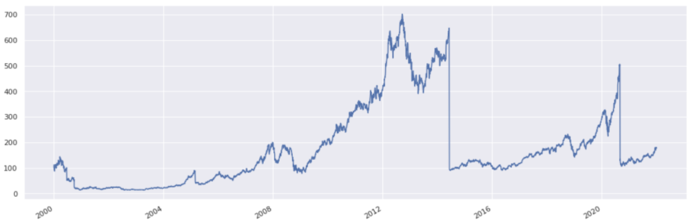
A pandas series or dataframe can be plotted by calling the plot method:
Input:
stock_history.plot()
Output:
<matplotlib.axes._subplots.AxesSubplot at 0x7fb826b4dcd0>
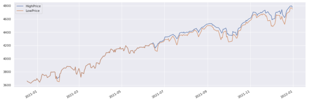
For a dataframe, the column names are automatically used to form the legend.
Input:
futures_data.plot()
Output:
<matplotlib.axes._subplots.AxesSubplot at 0x7fb826a69950>
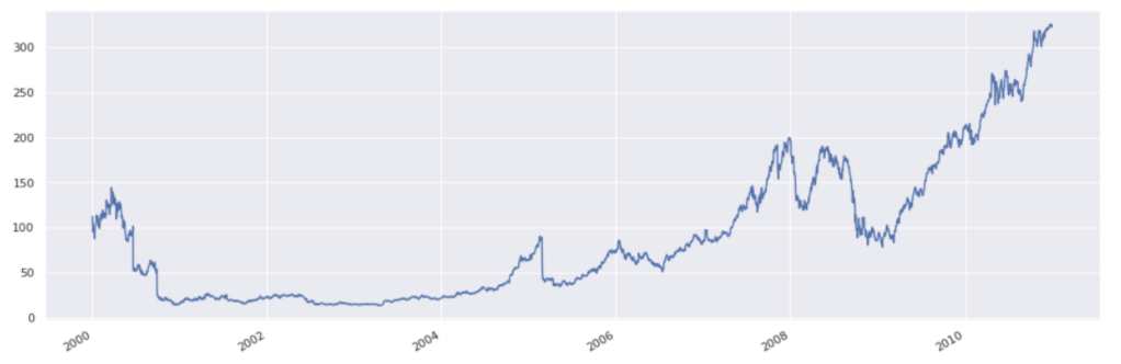
As filtering based on date returns another pandas series, or dataframe, the same plot method can be used on the result of filtering.
stock_history.loc[:'2010'].plot();
Computing returns#
Returns can be obtained from price series by using the pct_change method:
Input:
returns = stock_history.pct_change()
returns
Output:
2000-01-03 NaN
2000-01-04 -0.084310
2000-01-05 0.014634
2000-01-06 -0.086538
2000-01-07 0.047368
...
2021-12-27 0.022975
2021-12-28 -0.005767
2021-12-29 0.000502
2021-12-30 -0.006578
2021-12-31 -0.003535
Name: (LastPrice, EOD, 1000045.SINGLE_STOCK.TRADABLE), Length: 5536, dtype: float64
An equivalent way to obtain this would be to take the ratio of prices with one day forward shifted prices, and then subtract one:
Input:
stock_history.head()
Output:
2000-01-03 111.9375
2000-01-04 102.5000
2000-01-05 104.0000
2000-01-06 95.0000
2000-01-07 99.5000
Name: (LastPrice, EOD, 1000045.SINGLE_STOCK.TRADABLE), dtype: float64
Input:
stock_history.shift(1).head()
Output:
2000-01-03 NaN
2000-01-04 111.9375
2000-01-05 102.5000
2000-01-06 104.0000
2000-01-07 95.0000
Name: (LastPrice, EOD, 1000045.SINGLE_STOCK.TRADABLE), dtype: float64
Input:
stock_history / stock_history.shift(1) - 1
Output:
2000-01-03 NaN
2000-01-04 -0.084310
2000-01-05 0.014634
2000-01-06 -0.086538
2000-01-07 0.047368
...
2021-12-27 0.022975
2021-12-28 -0.005767
2021-12-29 0.000502
2021-12-30 -0.006578
2021-12-31 -0.003535
Name: (LastPrice, EOD, 1000045.SINGLE_STOCK.TRADABLE), Length: 5536, dtype: float64
Note: division is well defined and done on an element-by-element basis, matching on the index. The subtraction of one is vectorised (applied to all elements).
To compute log returns, apply np.log to the ratio of prices to shifted prices. This is relying on the vectorised way in which a function is applied to each element of the series:
Input:
log_returns = np.log(stock_history / stock_history.shift(1))
log_returns
Output:
2000-01-03 NaN
2000-01-04 -0.088078
2000-01-05 0.014528
2000-01-06 -0.090514
2000-01-07 0.046281
...
2021-12-27 0.022715
2021-12-28 -0.005784
2021-12-29 0.000502
2021-12-30 -0.006600
2021-12-31 -0.003542
Name: (LastPrice, EOD, 1000045.SINGLE_STOCK.TRADABLE), Length: 5536, dtype: float64
Dropping nan values#
The first entry in the returns series is a ‘nan’. No return can be computed for January 3rd 2000 as no prices prior to this date are available.
Input:
returns.iloc[0]
Output:
nan
Such values can be removed from pandas series and dataframes by calling the dropna method.
Calling this method does not alter the series or dataframe but returns a different series with nan values removed.
Input:
returns.dropna()
returns.head()
Output:
2000-01-03 NaN
2000-01-04 -0.084310
2000-01-05 0.014634
2000-01-06 -0.086538
2000-01-07 0.047368
Name: (LastPrice, EOD, 1000045.SINGLE_STOCK.TRADABLE), dtype: float64
Reassign returns to be the output from calling dropna:
Input:
returns = returns.dropna()
returns.head()
Output:
2000-01-04 -0.084310
2000-01-05 0.014634
2000-01-06 -0.086538
2000-01-07 0.047368
2000-01-10 -0.017588
Name: (LastPrice, EOD, 1000045.SINGLE_STOCK.TRADABLE), dtype: float64
To take a synthetic example, a dataframe with three columns is built as follows:
df = pd.DataFrame({
    'A': [1, 2, np.nan, np.nan],
    'B': [np.nan, 0, 0.5, np.nan],
    'C': [np.nan, np.nan, np.nan, np.nan]
})
df
The default behaviour of dropna is to remove any row containing at least one nan.
df.dropna()
The how parameter enables a requirement of every element in a row being nan before that row is removed.
df.dropna(how='all')
When performing operations on a dataframe there are two possible axes to apply the operation, as opposed to one for a series.
To apply an operation along the dataframe’s index set axis to 0, and to apply it along the dataframe’s columns set axis to 1.
In the following cell, any column whose values are all nan is dropped, by specifying axis to be 1. In this way the operation is performed along columns.
df.dropna(how='all', axis=1)
Note: none of these transformations is permanent.
df
To make such a transformation permanent the result can either be saved in a new variable or the inplace parameter can be used.
df_no_na = df.dropna(how='all', axis=1)
df_no_na
Outliers and sorting#
Plot returns:
Input:
returns.plot()
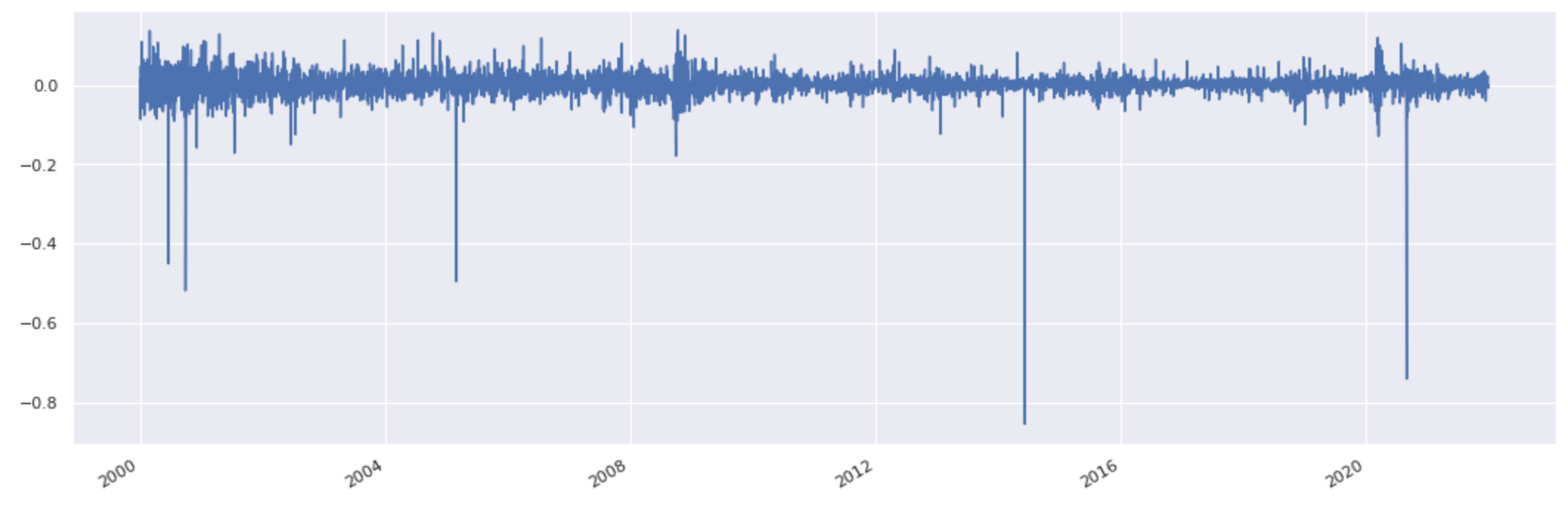
At first, some of these large downside moves may appear unexpected. To find out more the below cell sorts the data.
A pandas series can be sorted based on values by calling sort_values:
Input:
returns.sort_values()
Output:
2014-06-09 -0.854857
2020-08-31 -0.741522
2000-09-29 -0.518692
2005-02-28 -0.495899
2000-06-21 -0.450617
...
2008-11-24 0.125575
2001-04-19 0.128565
2004-10-14 0.131572
2000-03-01 0.136859
2008-10-13 0.139050
Name: (LastPrice, EOD, 1000045.SINGLE_STOCK.TRADABLE), Length: 5535, dtype: float64
Four of the five most negative returns are due to the fact that this price series is not adjusted for stock splits. An adjusted series can be fetched for any stock by calling adjusted_price_series.
stock_history = stock.adjusted_price_history(True, True)
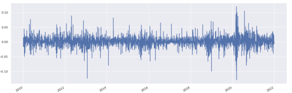
Recompute returns, drop nans and filter to data from 2010 onwards in one line. This sort of ‘piping’, or carrying out several operations in one line, can always be used with series and dataframes.
returns = stock_history.pct_change().dropna().loc['2010':]
returns.plot();
For a dataframe the method to sort is sort_values. A list of columns should then be provided to indicate the order of sorting preference.
df.sort_values(by=['B', 'A'])
Common statistics#
Common statistics like max, min, mean, median and standard deviation are easily obtained from a series or dataframe.
For the series case, it is clear what each of the statistics mean since there is only one axis to compute it over.
Input:
print(f'Max daily return: {round(100 * returns.max(), 2)}%')
print(f'Min daily return: {round(100 * returns.min(), 2)}%')
print(f'Mean daily return: {round(100 * returns.mean(), 2)}%')
print(f'Median daily return: {round(100 * returns.median(), 2)}%')
print(f'Standard deviation of daily returns: {round(100 * returns.std(), 2)}%')
Output:
Max daily return: 11.98%
Min daily return: -12.86%
Mean daily return: 0.13%
Median daily return: 0.1%
Standard deviation of daily returns: 1.77%
You can also use the built-in describe method to retrieve a collection of common statistics from the numeric data in a series or a dataframe. In particular, the result’s index will include count_,_ mean_,_ std_,_ min_,_ max as well as 25_,_ 50 and 75 percentiles.
Input:
returns.describe()
Output:
count    3021.000000
mean        0.001254
std         0.017667
min        -0.128647
25%        -0.007021
50%         0.001001
75%         0.010511
max         0.119808
dtype: float64
When the describe method is applied to object data, such as strings or timestamps, the resulting index will include count, unique, top and freq: top is the most common value, freq is the most common value’s frequency. Timestamps also include the first and last items.
returns.index.to_frame(name='Description').describe()
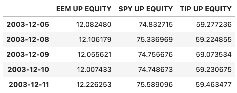
Dataframes can be built in a number of ways. One commonly used approach is to pass a dictionary to the pd.DataFrame constructor whose keys are strings and whose values are pd.Series objects:
etfs = ['EEM UP EQUITY', 'SPY UP EQUITY', 'TIP UP EQUITY']
dictionary_of_series = {
    etf: sig.obj.get(etf).adjusted_price_history(True, True)
    for etf in etfs
}
etf_data = pd.DataFrame(dictionary_of_series)
etf_data.head()
Remove any rows containing nan values.
etf_data = etf_data.dropna(how='any', axis=0)
etf_data.head()
Note: by default, aggregation operations on dataframes are done along the index (axis 0).
Input:
etf_returns.max()
Output:
EEM UP EQUITY    0.227699
SPY UP EQUITY    0.145198
TIP UP EQUITY    0.044537
dtype: float64
Input:
etf_returns.max(axis=0)
Output:
EEM UP EQUITY    0.227699
SPY UP EQUITY    0.145198
TIP UP EQUITY    0.044537
dtype: float64
Specifying axis to be 1 yields a series indexed by date with the relevant statistic computed over the list of ETFs on each day:
Input:
etf_returns.max(axis=1)
Output:
2003-12-08    0.006738
2003-12-09   -0.002555
2003-12-10    0.002660
2003-12-11    0.018224
2003-12-12    0.004587
                ...
2021-12-27    0.014152
2021-12-28   -0.000622
2021-12-29    0.001279
2021-12-30    0.011456
2021-12-31   -0.001237
Length: 4549, dtype: float64
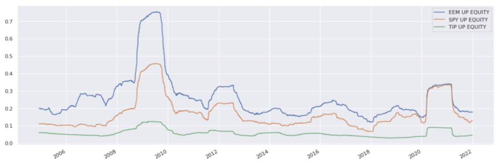
Rolling Volatility#
Compute rolling annualised volatilities over a 250 day window:
rolling_volatilities = etf_returns.rolling(window=250).std().dropna()
rolling_volatilities *= annualisation_factor
rolling_volatilities.plot();
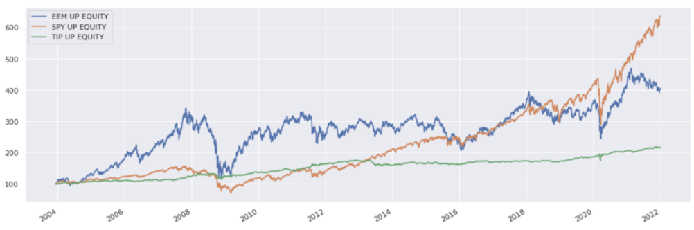
Scaling and reconstructing prices#
Rescale ETF prices to have the same starting point and plot:
scaled_etf_data = etf_data * 100 / etf_data.iloc[0]
scaled_etf_data.plot()
Reconstruct scaled price series from returns (except the first day):
etf_prices = (1 + etf_returns).cumprod()
etf_prices *= 100 / etf_prices.iloc[0]
etf_prices.plot()

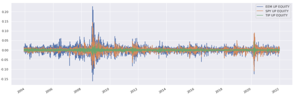
Further plotting#
Plot ETF returns together:
etf_returns.plot();
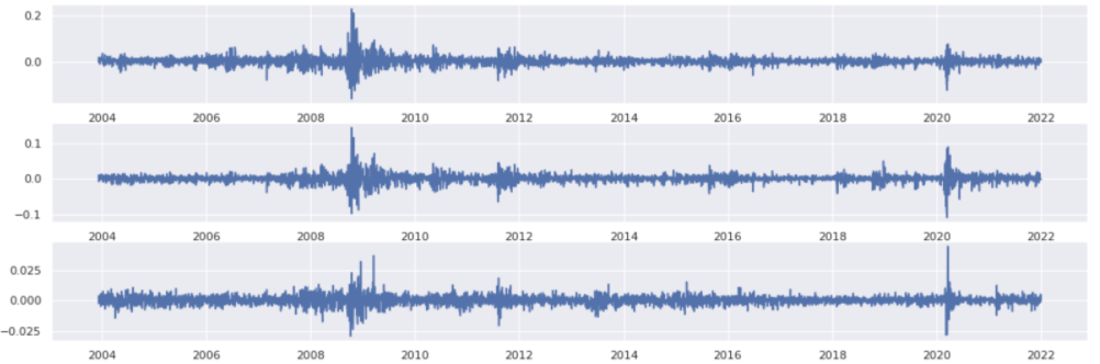
On separate axes:
fig, axes = plt.subplots(3)
for i, etf in enumerate(etf_returns):
    axes[i].plot(etf_returns[etf])
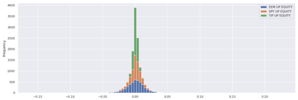
It is easy to show histograms as well as line plots:
etf_returns.plot(kind='hist', bins=100, stacked=True);
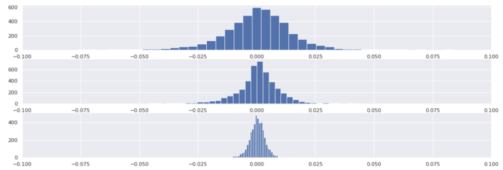
fig, axes = plt.subplots(3)
for i, etf in enumerate(etf_returns):
    axes[i].hist(etf_returns[etf], bins=100);
    axes[i].set_xlim(-0.1, 0.1)
Winsorisation example#
This sections shows an example of manually Winsorising returns at 3𝜎 for TIP ETF.
Fetch returns and compute an estimate of 𝜎:
tip_returns = etf_returns['TIP UP EQUITY'].copy()
sigma = tip_returns.std()
Compute the upper and lower cutoff values:
Input:
upper_cutoff = tip_returns.mean() + 3 * sigma
lower_cutoff = tip_returns.mean() - 3 * sigma
print(f'Upper cutoff: {round(100 * upper_cutoff, 2)}%')
print(f'Lower cutoff: {round(100 * lower_cutoff, 2)}%')
Output:
Upper cutoff: 1.17%
Lower cutoff: -1.13%
Check that the number of returns are larger than the upper cutoff:
Input:
upper_cutoff_count = tip_returns.loc[tip_returns > upper_cutoff].count()
upper_cutoff_count
Output:
25
A common indexing technique is being used here.
The following comparison returns a series of boolean with the same index as the tip_returns dataframe:
Input:
tip_returns > upper_cutoff
Output:
2003-12-08    False
2003-12-09    False
2003-12-10    False
2003-12-11    False
2003-12-12    False
              ...
2021-12-27    False
2021-12-28    False
2021-12-29    False
2021-12-30    False
2021-12-31    False
Name: TIP UP EQUITY, Length: 4549, dtype: bool
When passed to tip_returns this returns a series restricted to those index values where the condition was true:
Input:
tip_returns.loc[tip_returns > upper_cutoff].head()
Output:
2008-02-28    0.013242
2008-06-06    0.012236
2008-10-01    0.013234
2008-10-14    0.022872
2008-10-20    0.013722
Name: TIP UP EQUITY, dtype: float64
Calculate the proportion of returns impacted on the upside:
Input:
print(f'{round(100 * upper_cutoff_count / len(tip_returns), 2)}%')
Output:
0.55%
The same could be done on the downside.
To set different values on a slice of a dataframe it is good practice to use loc to access that particular slice and then set the new values:
tip_returns.loc[tip_returns > upper_cutoff] = upper_cutoff
tip_returns.loc[tip_returns < lower_cutoff] = lower_cutoff
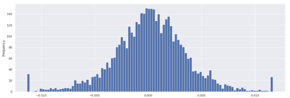
To see the impact of this winsorisation:
tip_returns.plot(kind='hist', bins=100);
Mapping for signal strategy#
This section shows an example of building a signal directly from a rolling futures strategy history time series and then using this signal as input to the SignalStrategy building block.
Import ES default Rolling Futures Strategy:
from sigtech.framework.default_strategy_objects.rolling_futures import es_index_front
es_rfs = es_index_front()
es_rfs.build()
Create constant +1 signal:
Input:
signal = 1 + 0 * es_rfs.history()
signal.head()
Output:
2010-01-04    1.0
2010-01-05    1.0
2010-01-06    1.0
2010-01-07    1.0
2010-01-08    1.0
Name: (LastPrice, EOD, USD ES INDEX LONG FRONT RF STRATEGY), dtype: float64
This is currently a pd.Series:
Input:
type(signal)
Output:
pandas.core.series.Series
Convert to a pd.DataFrame with column name using the tradable strategy name:
signal_df = signal.to_frame(name=es_rfs.name)
signal_df.head()
Input:
type(signal_df)
Output:
pandas.core.frame.DataFrame
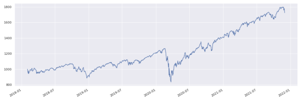
Build SignalStrategy from signal_df:
strategy = sig.SignalStrategy(
    currency='USD',
    start_date=dtm.date(2018, 2, 1),
    end_date=dtm.date(2021, 12, 1),
    signal_name=sig.signal_library.from_ts(signal_df).name
)
strategy.build()
strategy.history().plot();