Performance analytics

Learn how to generate and customize performance reports for your strategies.

A Primer notebook containing the code used in this page is available in the research environment. See Example notebooks for more information.

Pre-requisites

You have initialized a research environment. See Environment setup for instructions.

Importing Sigetch performance analytics

import sigtech.framework as sig
from sigtech.framework.analytics.performance.performance_report \
    import PerformanceReport, View, CustomView
import uuid
import datetime as dtm
import pandas as pd
import numpy as np
import seaborn as sns
sns.set(rc={'figure.figsize': (18, 6)})

if not sig.config.is_initialised():
    date = dtm.datetime(2020, 10, 30)
    sig.config.init(data_date=date, env_date=date)
    sig.config.set(sig.config.HISTORY_DATA_FILL_MISSING, True)

Create a basket of strategies

This step creates sample strategies for the performance report:

from sigtech.framework.default_strategy_objects.rolling_futures import *
from sigtech.framework.default_strategy_objects.rolling_futures_fx_hedged import *

us_basket = sig.BasketStrategy(
    currency='USD',
    start_date=dtm.date(2017, 1, 4),
    end_date=dtm.date(2020, 1, 4),
    constituent_names=[
        es_index_front().name,
        ty_comdty_front().name,
    ],
    weights=[0.5, 0.5],
    rebalance_frequency='EOM',
    ticker='USD USA BASKET {}'.format(str(uuid.uuid4())[:8]),
)

ge_basket = sig.BasketStrategy(
    currency='USD',
    start_date=dtm.date(2017, 1, 4),
    end_date=dtm.date(2020, 1, 4),
    constituent_names=[
        usd_gx_index_front().name,
        usd_rx_comdty_front().name,
    ],
    weights=[0.6, 0.4],
    rebalance_frequency='EOM',
    ticker='USD GERMANY BASKET {}'.format(str(uuid.uuid4())[:8]),
)

jp_basket = sig.BasketStrategy(
    currency='USD',
    start_date=dtm.date(2017, 1, 4),
    end_date=dtm.date(2020, 1, 4),
    constituent_names=[
        usd_nk_index_front().name,
        usd_jb_comdty_front().name,
    ],
    weights=[0.3, 0.7],
    rebalance_frequency='EOM',
    ticker='USD JAPAN BASKET {}'.format(str(uuid.uuid4())[:8]),
)

strategy1 = sig.BasketStrategy(
    currency='USD',
    start_date=dtm.date(2017, 1, 4),
    end_date=dtm.date(2020, 1, 4),
    constituent_names=[us_basket.name, ge_basket.name, jp_basket.name],
    weights=[0.6, 0.2, 0.2],
    rebalance_frequency='EOM',
    ticker='USD WORLD TOP_LEVEL BASKET {}'.format(str(uuid.uuid4())[:8])
)

strategy2 = sig.BasketStrategy(
    currency='USD',
    start_date=dtm.date(2017, 1, 4),
    end_date=dtm.date(2020, 1, 4),
    constituent_names=[ge_basket.name, jp_basket.name],
    weights=[0.7, 0.3],
    rebalance_frequency='EOM',
    ticker='USD WORLD TOP_LEVEL BASKET {}'.format(str(uuid.uuid4())[:8])
)

strategy3 = sig.BasketStrategy(
    currency='USD',
    start_date=dtm.date(2017, 1, 4),
    end_date=dtm.date(2020, 1, 4),
    constituent_names=[ge_basket.name, jp_basket.name],
    weights=[0.9, 0.1],
    rebalance_frequency='EOM',
    ticker='USD WORLD TOP_LEVEL BASKET {}'.format(str(uuid.uuid4())[:8])
)

Create a PerformanceReport from time series

A PerformanceReport can be created for a time series object. Method default_views() shows the report views enabled by default for this object:

Python

report0 = PerformanceReport(strategy1.history())
report0.default_views()

Output

[View('SUMMARY_SINGLE'),
 View('HISTORY'),
 View('PRESENTATION_PERF_TABLE'),
 View('SUMMARY_ROLLING_SERIES'),
 View('ROLLING_RISK_VOL'),
 View('ROLLING_RISK_SHARPE'),
 View('ROLLING_PLOTS'),
 View('MONTHLY_STATS'),
 View('MONTHLY_STATS_HEATMAP'),
 View('BENCHMARK_TABLE')]

Create a PerformanceReport from strategy

A PerformanceReport can also be created for a Strategy object. Method default_views() shows an extended list of report views enabled by default:

Input

report1 = PerformanceReport(strategy1)
report1.default_views()

Output

[View('SUMMARY_SINGLE'),
 View('HISTORY'),
 View('PRESENTATION_PERF_TABLE'),
 View('SUMMARY_ROLLING_SERIES'),
 View('ROLLING_RISK_VOL'),
 View('ROLLING_RISK_SHARPE'),
 View('POSITIONS_DF'),
 View('TURNOVER'),
 View('TURNOVER_STATS'),
 View('ROLLING_PLOTS'),
 View('MONTHLY_STATS'),
 View('MONTHLY_STATS_HEATMAP'),
 View('BENCHMARK_TABLE')]

Views

All built-in views can be accessed using the following syntax:

Input

View.TURNOVER

Output

View('TURNOVER')

Customised views can be accessed using the following syntax:

Input

View('Custom View')

Output

View('Custom View')

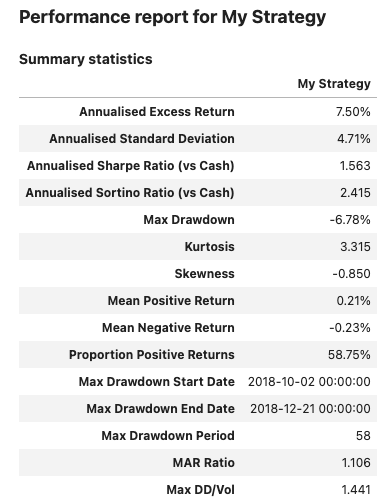
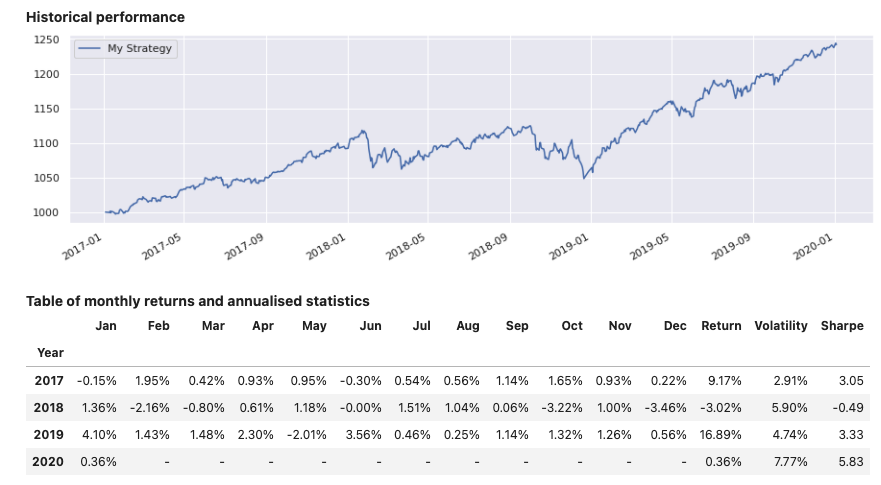
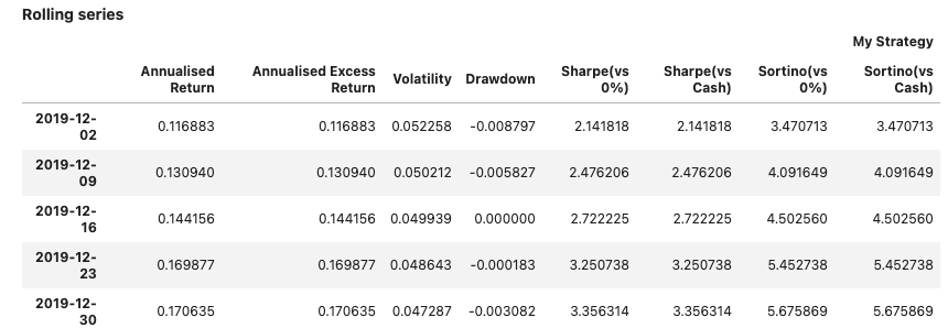
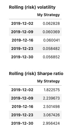
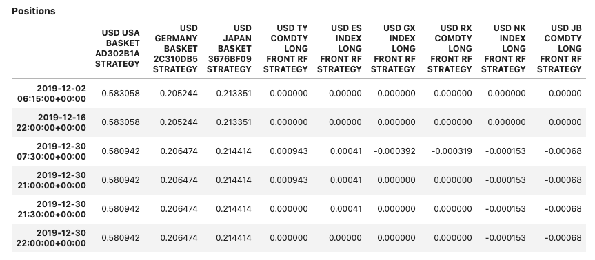
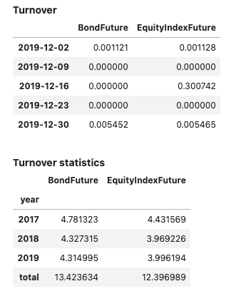
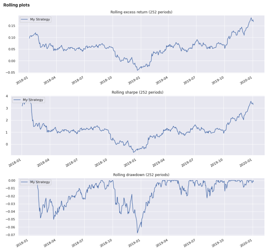
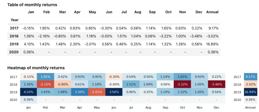
Display a report

Method report() will display the views enabled for the object used. Parameter dates can be specified to reduce the output size for tables showing daily data.

Input

few_dates = pd.date_range(dtm.date(2019, 12, 2), 
                          dtm.date(2020, 1, 1), freq='7d')
                          
report1 = PerformanceReport(strategy1, name='My Strategy', dates=few_dates)
report1.report()

Output

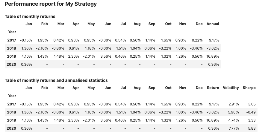
Specifying views when initializing PerformanceReport

Parameter views can be used to select a subset of the default views to display:

Input

report2 = PerformanceReport(strategy1,
                       name='My Strategy',
                       views=[View.MONTHLY_STATS,
                              View.PRESENTATION_PERF_TABLE],
                       dates=few_dates)
report2.views()

Output

[View('MONTHLY_STATS'), View('PRESENTATION_PERF_TABLE')]

Input

report2.report()

Output

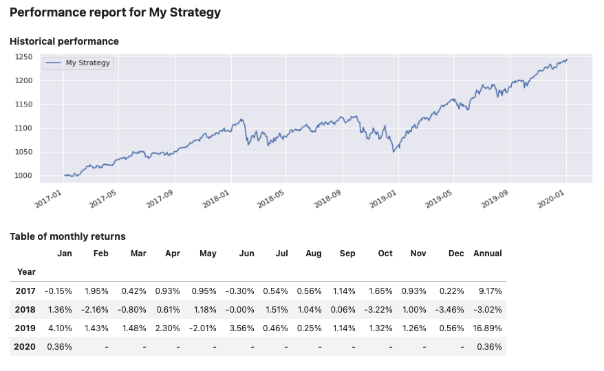
Use of arrange_views()

Within the same report, the order of views can also be re-arranged:

Input

report2.arrange_views([View.HISTORY, View.MONTHLY_STATS])
report2.report()

Output

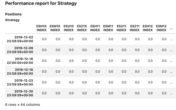
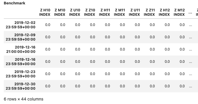
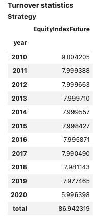
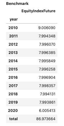
Add a benchmark strategy or time series

Parameter benchmark can be used to add a strategy or time series to the performance report. The following example uses one strategy as input object:

Input

s = es_index_front()
b = z_index_front()

report3 = PerformanceReport(s,
                       benchmark=b,
                       views=[View.POSITIONS_DF, View.TURNOVER_STATS],
                       dates=few_dates)
report3.report()

Output

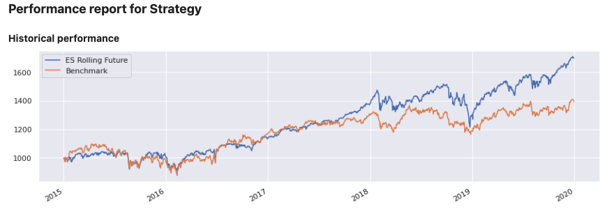
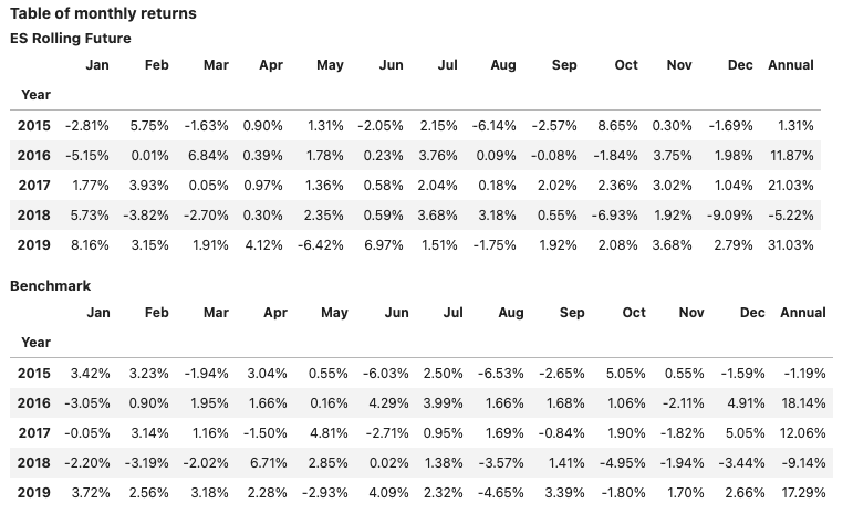
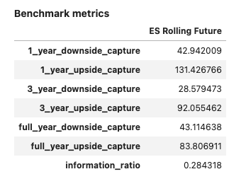
The same syntax is available for time series:

Input

ts = s.history().rename('ES Rolling Future').loc[
     dtm.date(2015, 1, 1):dtm.date(2020, 1, 1)]
ts_b = b.history()

report3 = PerformanceReport(ts,
                       benchmark=ts_b,
                       views=[View.HISTORY, View.MONTHLY_STATS,
                              View.BENCHMARK_TABLE])
report3.report()

Output

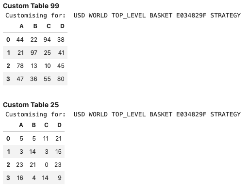
Add customised views

Customized views can be added to PerformanceReport by simply defining a new function. The following example defines two functions handling a DataFrame and a Pyplot graph:

# Define custom functions for view
def custom_table(args):
    # This function expects 2 parameters (Strategy, Integer)
    print('Customising for: ', args[0].name)
    df = pd.DataFrame(np.random.randint(0, args[1], size=(4, 4)),
                      columns=list('ABCD'))
    return df


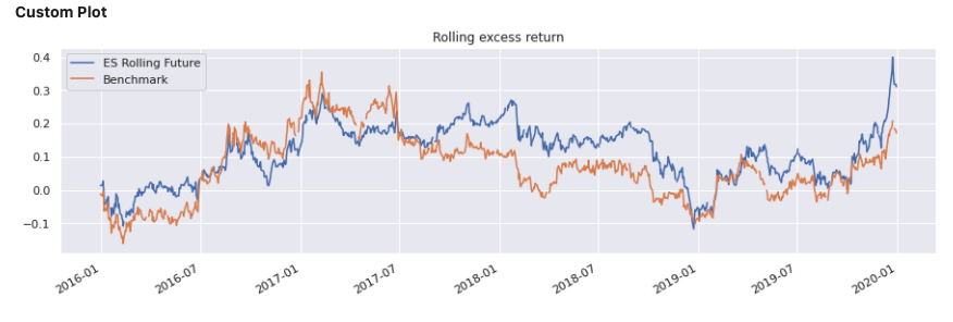
def custom_plot(args):
    # This function expects 1 parameter (PerformanceReport)
    import matplotlib.pyplot as plt
    args.rolling_stat('excess_return').plot(
        title="Rolling excess return", figsize=[15, 4])
    plt.show()
    return

A CustomView object helps wrapping the customised view and its parameters:

custom_view1 = CustomView(custom_table, params=[strategy1, 99],
                          name='Custom Table 99')
custom_view2 = CustomView(custom_table, params=[strategy1, 25],
                          name='Custom Table 25')
custom_view3 = CustomView(custom_plot, params=report3,
                          name='Custom Plot')

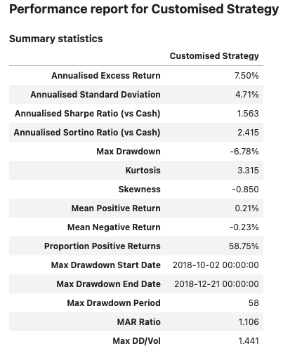
The customized views can now be added to the report:

Input

report3 = PerformanceReport(strategy1, name='Customised Strategy',
                       views=[View.SUMMARY_SINGLE])
report3.add_view(custom_view1)
report3.add_views([custom_view2, custom_view3])
report3.views()

Output

[View('SUMMARY_SINGLE'),
 View('Custom Table 99'),
 View('Custom Table 25'),
 View('Custom Plot')]

Input

report3.report()

Output

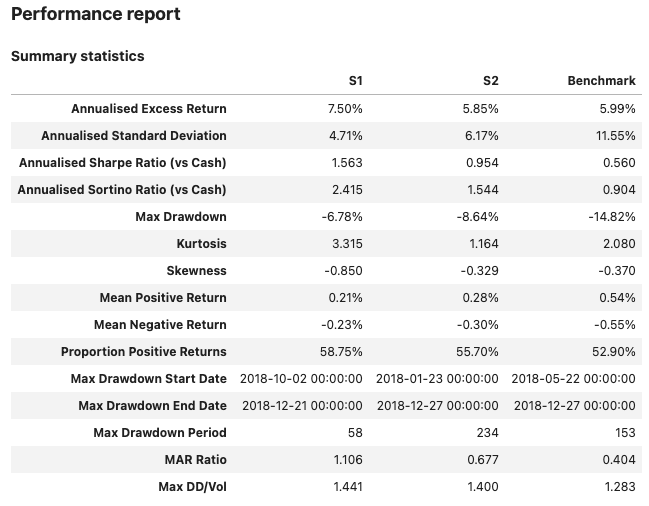
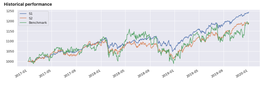
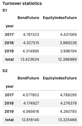
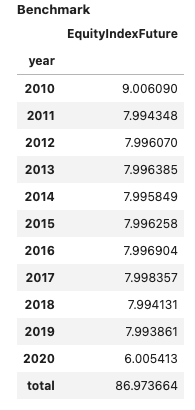
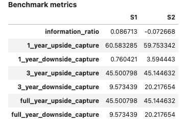
Support for multiple strategies

Reports for multiple strategies can be visualized by adding them to a list:

Input

report1 = PerformanceReport([strategy1, strategy2],
                       benchmark=b, name=['S1', 'S2'],
                       views=[View.SUMMARY_SINGLE, View.HISTORY,
                              View.TURNOVER_STATS, View.BENCHMARK_TABLE])
report1.report()

Output

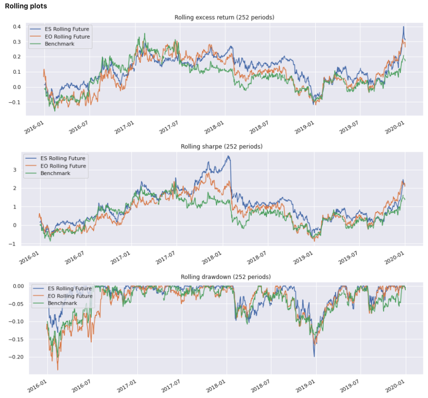
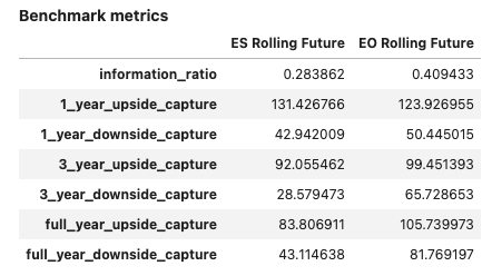
Support for multiple time series

Time series can be merged within a DataFrame object:

Input

ts1 = es_index_front().history().rename('ES Rolling Future').loc[
      dtm.date(2015, 1, 1):dtm.date(2020, 1, 1)]
ts2 = eo_index_front().history().rename('EO Rolling Future').loc[
      dtm.date(2015, 1, 1):dtm.date(2020, 1, 1)]
b = z_index_front().history()

ts_df = pd.concat({
    'ES Rolling Future': ts1,
    'EO Rolling Future': ts2,
}, axis=1)

rep = PerformanceReport(ts_df, benchmark=b,
                   views=[View.ROLLING_PLOTS, View.BENCHMARK_TABLE])
rep.report()

Output

Additional parameters for Performance Analytics

You can include currency based metrics in PerformanceReport. The following code block demonstrates how to include these views.

You can include currency based metrics in PerformanceReport. The following code block demonstrates how to include these views:

rfs = sig.RollingFutureStrategy(
    currency='USD',
    start_date=dtm.date(2020,1,1),
    contract_code='ES',
    contract_sector='INDEX',
    rolling_rule='front',
    fixed_contracts=1
)
rfs.build()

dates = pd.date_range('2021-01-04', '2021-12-01', freq='1W-MON')

sig.PerformanceReport(rfs, views=[sig.View.SUMMARY_SINGLE_CCY, sig.View.SUMMARY_ROLLING_CCY_SERIES], dates=dates).report()

rfs = sig.RollingFutureStrategy(
currency='USD',
start_date=dtm.date(2020,1,1),
contract_code='ES',
contract_sector='INDEX',
rolling_rule='front',
fixed_contracts=1
)
rfs.build()
dates = pd.date_range('2021-01-04', '2021-12-01', freq='1W-MON')
sig.PerformanceReport(rfs, views=[sig.View.SUMMARY_SINGLE_CCY, sig.View.SUMMARY_ROLLING_CCY_SERIES], dates=dates).report()

The aum argument allows you to pass a representative AUM figure. This is useful in strategies where initial_cash=0 as it avoids dividing by zero. Following on from the above code block, the use of this new argument is demonstrated below.

The aum argument allows you to pass a representative AUM figure. This is useful in strategies where initial_cash=0 as it avoids dividing by zero. The use of this argument is demonstrated in the following code block:

sig.PerformanceReport(rfs, dates=dates, views=[sig.View.SUMMARY_SINGLE]).report()

first_contract = sig.obj.get(rfs.rolling_table.rolled_in_contract.iloc[0])
first_contract_value = first_contract.history().asof(rfs.start_date.strftime("%Y-%m-%d")) * first_contract.contract_size

sig.PerformanceReport(
    rfs, 
    dates=dates, 
    views=[sig.View.SUMMARY_SINGLE], 
    aum=first_contract_value
).report()

sig.PerformanceReport(rfs, dates=dates, views=[sig.View.SUMMARY_SINGLE]).report()
first_contract = sig.obj.get(rfs.rolling_table.rolled_in_contract.iloc[0])
first_contract_value = first_contract.history().asof(rfs.start_date.strftime("%Y-%m-%d")) * first_contract.contract_size
sig.PerformanceReport(
rfs,
dates=dates,
views=[sig.View.SUMMARY_SINGLE],
aum=first_contract_value
).report()

In addition, you can generate a PerformanceReport with compounded metrics by passing compound_metrics=True . The below code block demonstrates this feature by building on the examples provided above.

You can also generate a PerformanceReport with compounded metrics by passing compound_metrics=True. The following code block demonstrates this feature by building on the examples provided above:\

sig.PerformanceReport(
    rfs, 
    dates=dates[-5:], 
    views=[sig.View.SUMMARY_ROLLING_SERIES], 
    aum=first_contract_value,
    compound_metrics=True
).report()

sig.PerformanceReport(
rfs,
dates=dates[-5:],
views=[sig.View.SUMMARY_ROLLING_SERIES],
aum=first_contract_value,
compound_metrics=True
).report()