Default strategies

This page shows the default strategies that are available within the framework. The strategy objects are intended to speed up the process of strategy creation as common strategies can be called with a single line of code.

Note: the default strategies described in this section are unrelated to the example notebooks which can be access in the research environment. For more information, see Example notebooks.

Available default strategies

• Default Rolling Future Strategies

• Default Rolling FX Forward Strategies

• Default Single Stock Reinvestment Strategies

• Default ETF Reinvestment Strategies

• Default Rolling Option Strategies

• Default Rolling Bond Strategies

• Default Rolling Swap Strategies

• Default Rolling FX-hedged Swap Strategies

Example use of default strategies

Setting up your environment takes three steps:

• Import the relevant internal and external libraries

• Configure the environment parameters

• Initialise the environment

import sigtech.framework as sig
import datetime as dtm
import seaborn as sns

sns.set(rc={'figure.figsize':(18,6)})
sig.config.init();

Learn more: setting up the environment.

To use a default strategy within the platform, they must be imported. An example for RollingFutureStrategy default strategies is shown here:

from sigtech.framework.default_strategy_objects.rolling_futures import *

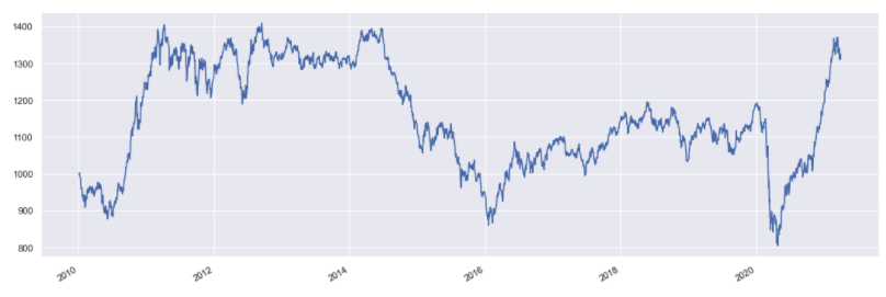
The following example shows how these default strategies are used to create a simple BasketStrategy object of several RollingFutureStrategy objects:

assets = {
    'Treasury Futures (TY)': ty_comdty_front().name,
    'Corn Futures (C)': c_comdty_f_0().name,
    'Soybean Futures (S)': s_comdty_f_0().name,
    'Sugar Futures (SB)': sb_comdty_f_0().name,
    'Cotton Futures (CT)': ct_comdty_f_0().name,
    'Live Cattle Futures (LC)': lc_comdty_f_0().name,
    'Soybean Oil Futures (BO)': bo_comdty_f_0().name,
    'Brent Crude Futures (CO)': co_comdty_f_0().name,
    'Gas Oil Futures (QS)': qs_comdty_f_0().name,
    'Heating Oil Futures (HO)': ho_comdty_f_0().name,
    'S&P Futures (ES)': es_index_front().name,
    'Nasdaq Futures (NQ)': nq_index_front().name
}

Input:

sig.BasketStrategy(
    constituent_names = assets.values(),
    start_date = dtm.date(2010, 1, 4),
    currency = 'USD',
    weights = [1 / len(assets.values())] * len(assets.values()),
    rebalance_frequency = '1M'
).history().plot()

Output:

See also:

• Example notebooks