Equity factor optimization#
This page demonstrates the tools available to fit factor exposures for the optimization of an equities portfolio.
Learn more: Example notebooks
Environment#
There are three steps to setting up your environment:
Import the relevant internal and external libraries
Configure the environment parameters
Initialise the environment
import numpy as np
import pandas as pd
import seaborn as sns
import datetime as dtm

sns.set(rc={'figure.figsize': (18, 6)})

import sigtech.framework as sig
from sigtech.framework.analytics.optimization.optimization_problem import TermTypes, MetricTypes
from sigtech.framework.default_strategy_objects.single_stock_strategies import get_single_stock_strategy

if not sig.config.is_initialised():
    env = sig.init(env_date=dtm.date(2022, 1, 4))

START_DATE = dtm.date(2021, 1, 4)
Learn more: setting up the environment
Set an initial portfolio #
You can create strategies to buy and sell single stock strategy objects.
The following code block filters the top 20 SPX INDEX constituents by MARKETCAP:
Input:
equity_filter = sig.EquityUniverseFilter('SPX INDEX')

equity_filter.add('MARKETCAP', 'Top', 20, 'Daily')

universe = equity_filter.apply_filter(START_DATE).iloc[0]
Output:
['1001489.SINGLE_STOCK.TRADABLE',
 '1000045.SINGLE_STOCK.TRADABLE',
 '1001962.SINGLE_STOCK.TRADABLE',
 '1083049.SINGLE_STOCK.TRADABLE',
 '1031651.SINGLE_STOCK.TRADABLE',
 '1070370.SINGLE_STOCK.TRADABLE',
 '1014425.SINGLE_STOCK.TRADABLE',
 '1039790.SINGLE_STOCK.TRADABLE',
 '1003331.SINGLE_STOCK.TRADABLE',
 '1013816.SINGLE_STOCK.TRADABLE',
 '1000896.SINGLE_STOCK.TRADABLE',
 '1035463.SINGLE_STOCK.TRADABLE',
 '1004551.SINGLE_STOCK.TRADABLE',
 '1012437.SINGLE_STOCK.TRADABLE',
 '1010576.SINGLE_STOCK.TRADABLE',
 '1010398.SINGLE_STOCK.TRADABLE',
 '1003282.SINGLE_STOCK.TRADABLE',
 '1011879.SINGLE_STOCK.TRADABLE',
 '1006879.SINGLE_STOCK.TRADABLE',
 '1011408.SINGLE_STOCK.TRADABLE']
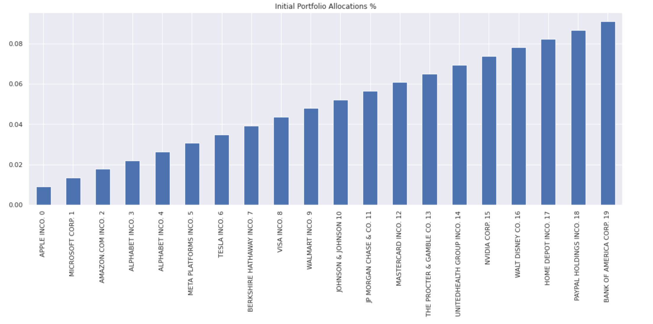
You can then define an initial portfolio. In the following example linearly increasing weights are applied to the 20 large cap stocks:
company_names = [f"{sig.obj.get(x).company_name} {n}" for n, x in enumerate(universe)]

pf_ts = pd.Series(index=company_names, data=np.linspace(0.1,1,20))

pf_ts = pf_ts / pf_ts.sum()

pf_ts.plot(kind='bar', title='Initial Portfolio Allocations %');
To create the reinvestment strategies and calculate their corresponding returns:
rs = [get_single_stock_strategy(ss) for ss in universe]

universe_mapping = {ss: f'{ss} REINV STRATEGY' for ss in universe}

single_stock_returns = {s.name: s.history().pct_change().dropna()  for s in rs}

pf_ts.index = universe_mapping.values()
Fit factor exposures#
To calculate your static portfolio’s exposure to the Fama-French factors—market risk, small minus big, high minus low—fit these factors to your portfolio’s stock returns:
Learn more: Factor exposures
Load factor data#
factor_series = sig.obj.get('US 3F_DAILY FAMA-FRENCH INDEX').history_df(['mkt_rf', 'smb', 'hml'])

factor_series.head()
Create factor exposure#
factor_exposure = sig.FactorExposures()

factor_exposure.add_regression_factors(factor_series, names=['MKT', 'SMB', 'HML'])

factor_exposure.fit(single_stock_returns);
Optimisation#
The factor exposure object is used to provide information to an optimiser. This optimisation is specified by an OptimizationProblem object and performed using the Optimizer class.
Interactive optimiser#
Use the interactive optimisation interface to construct an optimisation problem and explore the results:
int_port_opt = sig.InteractivePortfolioOptimizer(
    portfolio=pf_ts,
    targets_df=pd.concat(single_stock_returns, axis=1),
    factor_exposure_object=factor_exposure
)

int_port_opt
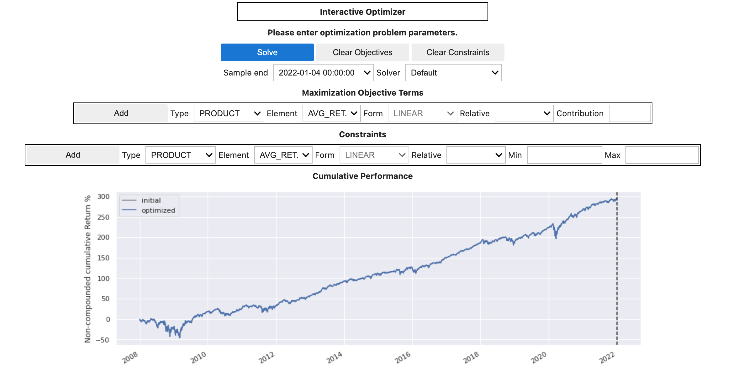
The interface allows you to test different static optimisations and retrieve the GUI’s current active OptimizationProblem object:
problem = int_port_opt.optimization_problem
Defining an optimisation #
A problem can also be defined by code. The following example sets up an optimization problem, defining objectives and bounds (also known as constraints):
# Create an optimization problem
problem = sig.OptimizationProblem()

# Add an objective to minimize the exposure to the market factor
problem.set_optimizer_objective(TermTypes.EXPOSURE, element='MKT', metric=MetricTypes.SQUARE, value=-0.0001)

# Add an objective to minimize the variance
problem.set_optimizer_objective(TermTypes.VARIANCE, element='FULL', metric=MetricTypes.VARIANCE, value=-1)

# Add a constraint to go long only
problem.set_optimizer_bounds(TermTypes.WEIGHT, element='ALL', metric=MetricTypes.LINEAR, min_value=0)

# Add a constraint for 100% exposure
problem.set_optimizer_bounds(TermTypes.WEIGHT, element='SUM_', metric=MetricTypes.LINEAR, min_value=1, max_value=1)
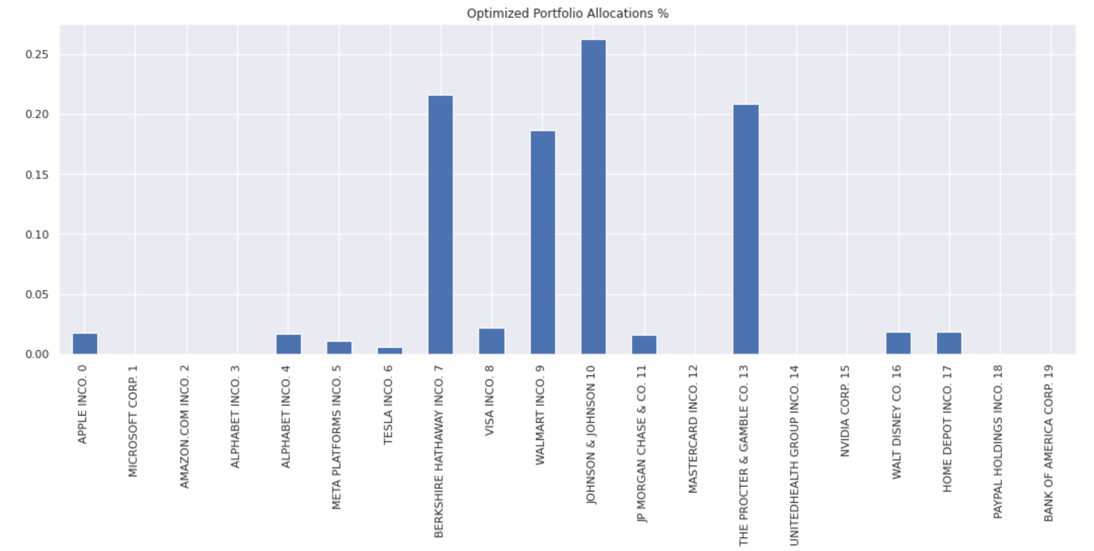
Running the problem with the Optimizer returns and plots the new optimized weights:
# Run optimization
optimizer = sig.Optimizer(factor_exposure, problem)

result = optimizer.calculate_optimized_weights()

result.index = company_names

result.plot(kind='bar', title='Optimized Portfolio Allocations %');
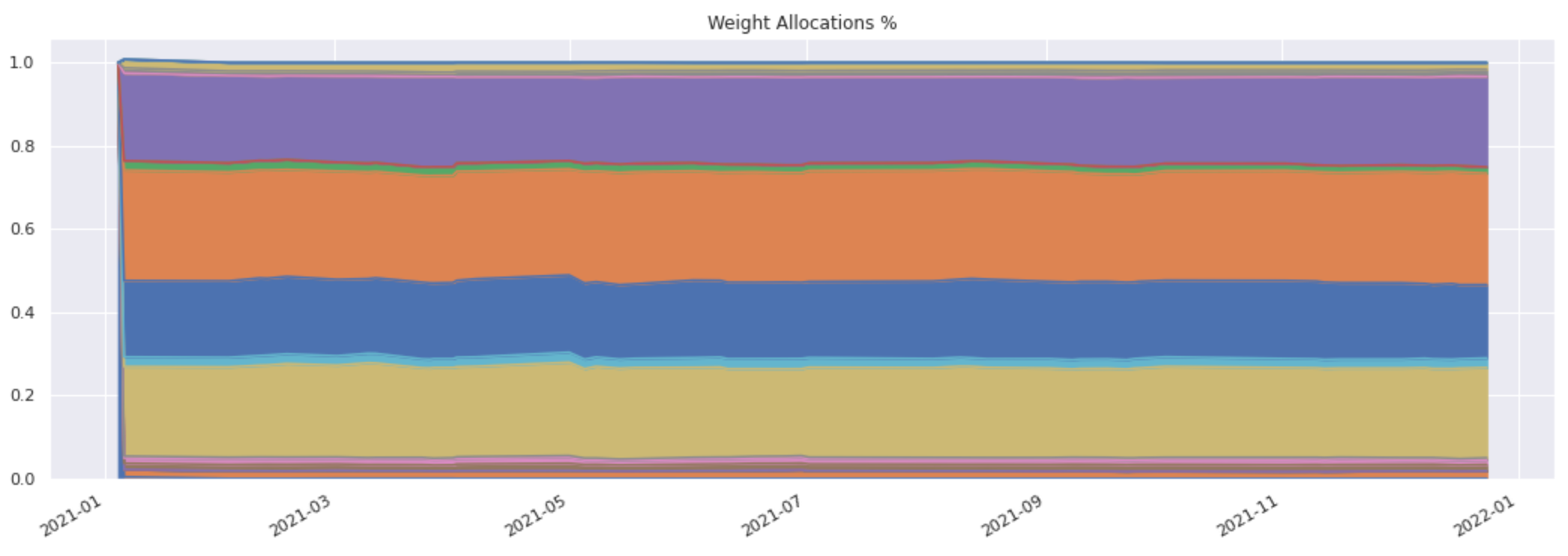
Rolling optimisation#
Once defined, the optimisation can be run on a rolling basis as part of a SignalStrategy or EquityFactorBasket using the factor_optimized_allocations allocation function.
Define a monthly rebalance schedule and construct an equally weighted portfolio by applying a single unit of weights to each reinvestment strategy in your signal DataFrame:
rebal_dates = sig.SchedulePeriodic(
START_DATE, env.asofdate,
'NYSE(T) CALENDAR', frequency='EOM'
).all_data_dates()
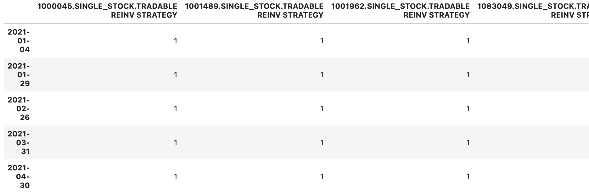
signal_df = pd.DataFrame({s.name: 1 for s in rs}, index=rebal_dates)
signal_df.head()
Then define your optimisation to be run on each rebalance date as part of your SignalStrategy:
opt_rolling_holdings = sig.SignalStrategy(
    currency='USD',
    start_date=START_DATE,
    use_signal_for_rebalance_dates=True,
    signal_name=sig.signal_library.core.from_ts(signal_df).name,
    allocation_function=sig.signal_library.allocation.optimized_allocations,
    allocation_kwargs={'factor_exposure_object': factor_exposure,
                       'optimization_problem': problem,
                       'instrument_mapping': universe_mapping}
)

opt_rolling_holdings.build()
opt_rolling_holdings.inspect.weights_df().abs().plot(kind='area', legend=False, title='Weight Allocations %');