Parameter analysis

This page shows how one might go about varying parameters in a strategy, and calculate the resulting Sharpe from each of the parameter runs.

The example is based around simple momentum and mean reversion strategies on the NY Harbor Heating Oil (HO COMDTY) Rolling Future Strategy.

Learn more: Example notebooks

Environment

This section will import relevant internal and external libraries, as well as setting up the platform environment.

Learn more: Environment setup

import sigtech.framework as sig
from sigtech.framework.analytics.performance.metrics import sharpe_ratio

import datetime as dtm
import pandas as pd
import numpy as np
import seaborn as sns
import matplotlib.pyplot as plt

sns.set(rc={'figure.figsize': (18, 6)})

if not sig.config.is_initialised():
    sig.config.init()
    sig.config.set(sig.config.HISTORY_SCHEDULE_BUILD_FROM_DATA, True)

Momentum: varying window length

A RollingFutureStrategy object of the NY Harbor Heating Oil contract is created:

Learn more: Rolling Future Strategy

ho_rf_usd_strat = sig.RollingFutureStrategy(
    currency='USD',
    start_date=dtm.date(2010, 1, 4),
    contract_code='HO',
    contract_sector='COMDTY',
    rolling_rule='F_0',
    monthly_roll_days='1:10'
)

Define a function to construct a momentum strategy with a custom window length:

@sig.remote
def momentum_strategy_sharpe(underlying_obj_name: str, window_length: int):
    ''' Constructs a SMA-based momentum strategy with a given window length.'''

    # Get return
    signal_ts = sig.obj.get(underlying_obj_name).history().diff(window_length)

    # Create df with column name equal to underlying object name
    signal_ts = pd.DataFrame({underlying_obj_name: signal_ts})

    # Get sign of returns
    signal_ts = np.sign(signal_ts).dropna()

    # Create signal object, can be passed around between researchers
    signal_obj = sig.signal_library.from_ts(signal_ts)

    signal_strategy = sig.SignalStrategy(
        start_date=dtm.date(2010, 1, 4),
        currency='USD',
        signal_name=signal_obj.name,
        rebalance_frequency='EOM',
        allocation_function=sig.signal_library.allocation.identity,
        leverage=1,
    )

    return sharpe_ratio(signal_strategy.history())

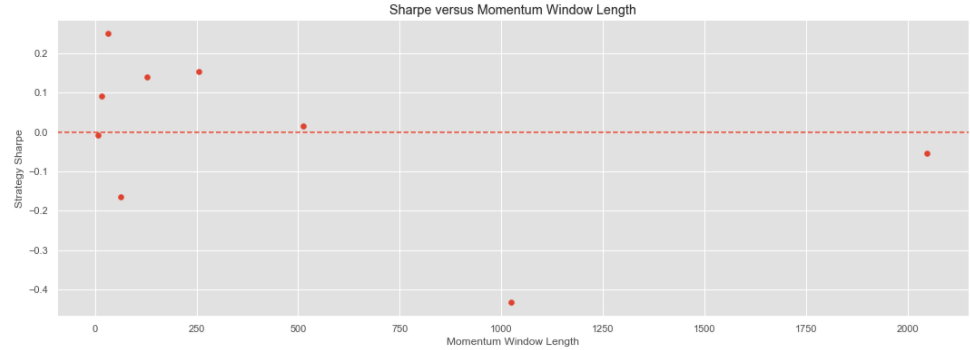
Use this function to construct a number of strategies and plot their Sharpe ratios:

plt.style.use('ggplot')

# Generate window lengths as powers of 2
x = [2 ** i for i in range(3, 12)]

# Generate resulting Sharpe ratios
ho_rf_usd_strat.build()
y = sig.calc_remote([momentum_strategy_sharpe(ho_rf_usd_strat.name, w) for w in x])

# Plot results and annotate chart
fig, ax = plt.subplots()
ax.scatter(x, y)
ax.set_title('Sharpe versus Momentum Window Length')
ax.set_xlabel('Momentum Window Length')
ax.set_ylabel('Strategy Sharpe')
ax.axhline(y=0., linestyle='--');

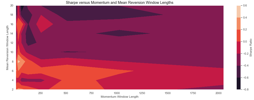
Momentum and Mean Reversion: varying window lengths

A 2D surface from varying both Momentum and Mean Reversion windows is created in the following example.

First, define a function to calculate the Sharpe for a combined Momentum and Mean Reversion strategy:

@sig.remote
def mmr_strategy_sharpe(
        underlying_obj_name: str,
        momentum_window_length: int,
        meanrev_window_length: int):
    """ Constructs a combined Momentum and Mean Reversion strategy on a given underlying. """

    # Identical lengths of windows will cancel out, ignore them
    if momentum_window_length == meanrev_window_length:
        return 0.

    # Get history of underlyer
    obj_history = sig.obj.get(underlying_obj_name).history()

    # Create momentum and mean reversion signals and combine them
    signal_momentum = obj_history.pct_change().rolling(
        window=momentum_window_length).mean()
    signal_meanrev = -obj_history.pct_change().rolling(window=meanrev_window_length).mean()
    signal_ts = signal_momentum + signal_meanrev

    # Create df with column name equal to underlying object name
    signal_ts = pd.DataFrame({underlying_obj_name: signal_ts})

    # Get sign of returns
    signal_ts = np.sign(signal_ts).dropna()

    # Create signal object, can be passed around between researchers
    signal_obj = sig.signal_library.from_ts(signal_ts)

    strategy = sig.SignalStrategy(
        start_date=dtm.date(2010, 1, 4),
        currency='USD',
        signal_name=signal_obj.name,
        rebalance_frequency='EOM',
        allocation_function=sig.signal_library.allocation.identity,
        leverage=1,
    )

    return sharpe_ratio(strategy.history())

Then use this function to construct a number of strategies and plot their Sharpe ratios on a 2D plot:

# Generate window lengths in specific ranges
mom_ws = [2 ** i for i in range(3, 12)]
mr_ws = range(2, 21, 2)

# Generate resulting Sharpe ratios in a 2D array
sharpes = sig.calc_remote(
    [
        mmr_strategy_sharpe(
            underlying_obj_name=ho_rf_usd_strat.name,
            momentum_window_length=w1,
            meanrev_window_length=w2
        )
        for w2 in mr_ws for w1 in mom_ws
    ]
)
z = np.matrix(np.array(sharpes).reshape(len(mr_ws), len(mom_ws)))

# Plot results and annotate chart
fig, ax = plt.subplots()
plot = ax.contourf(mom_ws, mr_ws, z)
ax.set_title('Sharpe versus Momentum and Mean Reversion Window Lengths')
ax.set_xlabel('Momentum Window Length')
ax.set_ylabel('Mean Reversion Window Length')
cbar = fig.colorbar(plot, ax=ax)
cbar.ax.set_ylabel('Sharpe Ratio');