Portfolio optimisation

This section provides examples of the optimisers available and how they can be used.

The following example will optimise a basket of large cap stocks through different objectives and constraints, comparing each problem to a minimum variance portfolio.

Learn more: example notebooks

Environment

This section imports the relevant internal and external libraries, and sets up the platform environment.

Learn more: setting up the environment.

import numpy as np
import pandas as pd
import seaborn as sns
from uuid import uuid4
import datetime as dtm
from tqdm.notebook import tqdm
import matplotlib.pyplot as plt

sns.set(rc = {'figure.figsize': (18, 6)})

import sigtech.framework as sig
from sigtech.framework.default_strategy_objects.single_stock_strategies import get_single_stock_strategy

if not sig.config.is_initialised():
    env = sig.init(env_date=dtm.date(2022, 1, 4))

Define universe

The following example considers a basket of large cap stocks from the SPX index. We start by building a reinvestment strategy for each stock:

START_DATE = dtm.date(2020, 1, 4)

equity_filter = sig.EquityUniverseFilter('SPX INDEX')

equity_filter.add('Market Cap', 'Top', 10, frequency='Quarterly')

universe = equity_filter.apply_filter(START_DATE).iloc[0]

rs = [get_single_stock_strategy(ss) for ss in universe]

The total returns are then computed for each stock and mapped to company names:

company_names = list(set([sig.obj.get(ss).company_name for ss in universe]))

single_stock_returns = {n: s.history().pct_change().dropna() for s, n in zip(rs, company_names)}

single_stock_returns_df = pd.concat(single_stock_returns, 1)[START_DATE:]

universe_mapping = {n: f'{ss} REINV STRATEGY' for ss, n in zip(universe, company_names)}

single_stock_mapping = {n: ss for ss, n in zip(universe, company_names)}

Helper functions

Two variables are defined to store our optimised weights and strategy objects for each problem we solve:

STRATEGIES = {}
PROBLEM_WEIGHTS = {}

Two helper functions are also defined. run_optimisation_on_basket will build our basket of stocks via a SignalStrategy using weights stored in PROBLEM_WEIGHTS for each problem name:

def run_optimisation_on_basket(problem_name: str):
    """
    Build the basket as a signal strategy with the optimised weights for the given problem_name
    The optimised weights are retrieved from the problem_weights dictionary
    """

    weights = PROBLEM_WEIGHTS[problem_name]
    signal_df = weights.to_frame(START_DATE).T
    
    optimised_signal_strategy = sig.SignalStrategy(
        currency='USD',
        start_date=START_DATE,
        signal_name=sig.signal_library.core.from_ts(signal_df).name,
        rebalance_frequency='EOM',        
        convert_long_short_weight=False,
        instrument_mapping=universe_mapping,
        ticker=f'{problem_name.upper()} OPTIMISED BASKET {str(uuid4())[:4]}'
    )
    
    optimised_signal_strategy.build()
    
    STRATEGIES[problem_name] = optimised_signal_strategy
    

plot_optimisation_results plots visualisations to illustrate the optimised weights and performance of the problem, relative to a minimum variance portfolio:

def plot_optimisation_results(problem_name: str):
    """
    Plot the weights for each holding and the resulting basket performance.
    If the problem name != "Min Variance", add Min Variance strategy to the plots for comparison.
    """
    
    return_ts = STRATEGIES[problem_name].history()
    weights = PROBLEM_WEIGHTS[problem_name]

    fig, (ax1, ax2) = plt.subplots(1, 2)

    weights.plot(ax=ax1, kind='bar', label=problem_name)
    return_ts.plot(ax=ax2, label=problem_name)
    
    mv = 'Min Variance'
    if problem_name != mv:
        min_var_return_ts = STRATEGIES[mv].history()
        min_var_weights = PROBLEM_WEIGHTS[mv]
        
        min_var_weights.plot(ax=ax1, kind='bar', fill=False, edgecolor='C1', ls='--', label=mv)
        min_var_return_ts.plot(ax=ax2, alpha=0.6, label=mv)
        
        ax1.legend()
        ax2.legend()
    
    return ax1, ax2

Optimisations

Optimisers are built through the sig.PortfolioOptimizer class, which acts as a wrapper around the Optimizer class.

The methods on this wrapper will build an OptimizationProblem object, adding the necessary constraints and objectives, and running it through Optimizer via the calculate_weights method.

Users are encouraged to use the wrapper, as it provides a more efficient interface, but can equally define their own OptimisationProblems at a lower level, as shown in Equity factor optimisation.

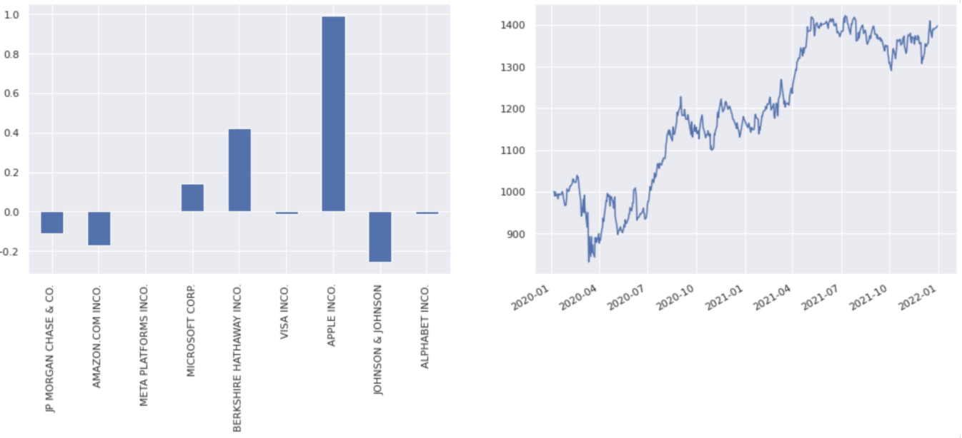
Minimum variance

PortfolioOptimizer is instantiated and an objective is added to minimise returns variance. A constraint is then added to ensure the portfolio weights sum to 100%:

min_var_opt = sig.PortfolioOptimizer().require_minimum_variance()

min_var_opt.require_fully_invested()

PROBLEM_WEIGHTS['Min Variance'] = min_var_opt.calculate_weights(single_stock_returns_df)

run_optimisation_on_basket('Min Variance')

plot_optimisation_results('Min Variance');

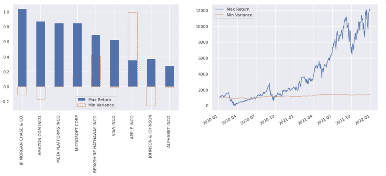
Maximum return

max_return_opt = sig.PortfolioOptimizer().require_maximum_return()

# This would be un-bound if we didn't add the L2 penalty
max_return_opt = max_return_opt.require_weights_l2_penalty(value=1e-3)

# Can set custom maximum return in .require_maximum_return() via the expected_returns= parameter

PROBLEM_WEIGHTS['Max Return'] = max_return_opt.calculate_weights(single_stock_returns_df)

run_optimisation_on_basket('Max Return')

plot_optimisation_results('Max Return');

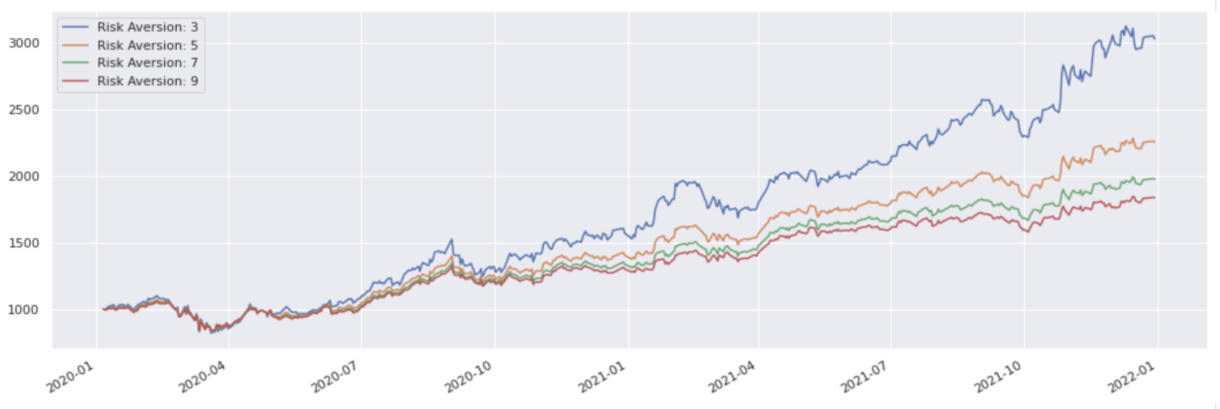
Mean-variance

The following function optimises our basket through require_mean_variance, given a risk aversion:

risk_aversions = [3, 5, 7, 9]

def mean_variance_weights(risk_aversion):
    problem_name = f'Mean Variance - {risk_aversion}'
    
    mean_var_opt = sig.PortfolioOptimizer().require_mean_variance(risk_aversion=risk_aversion)
    
    mean_var_opt.require_fully_invested()
    
    PROBLEM_WEIGHTS[problem_name] = mean_var_opt.calculate_weights(single_stock_returns_df)
    
    run_optimisation_on_basket(problem_name)
    
    optimised_return_ts = STRATEGIES[problem_name].history()
    
    return optimised_return_ts

mean_var_returns =  {f'Risk Aversion: {i:.0f}' : mean_variance_weights(i) for i in risk_aversions}

pd.concat(mean_var_returns, 1).plot();

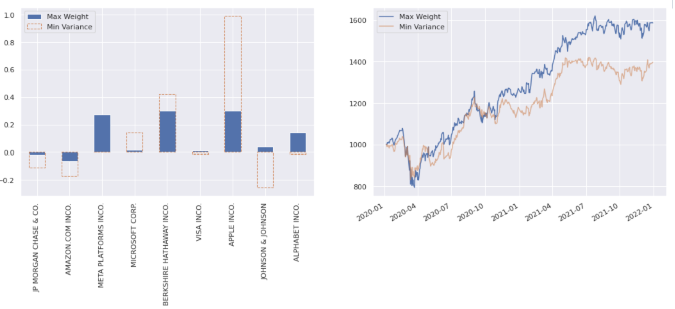
Maximum stock weight

The minimum variance is optimised in the following example, but with a max weight of 30% in a single holding through require_weight_limit:

max_stock_weight = sig.PortfolioOptimizer().require_weight_limit(max_value=0.3)

max_stock_weight.require_minimum_variance()

max_stock_weight.require_fully_invested()

PROBLEM_WEIGHTS['Max Weight'] = max_stock_weight.calculate_weights(single_stock_returns_df)

run_optimisation_on_basket('Max Weight')

plot_optimisation_results('Max Weight');

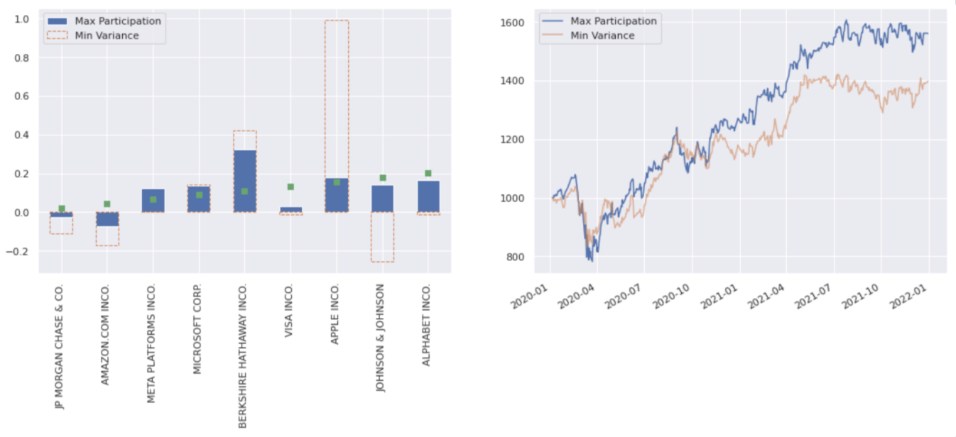
Maximum participation

The weight change, of the portfolio instruments to a percent of median daily volume, can be limited.

Note: this requirement cannot be used with the SignalStrategy allocation setup as the identity of all assets in the portfolio needs to be known before accessing the MDVs. This requirement can only be used on a step-by-step basis.

An example initial weights is generated to rebalance from:

initial_weights = pd.Series(index=company_names, data=np.linspace(0.1,1,9)) / 4.95

The require_limited_participation method is used with a max participation of 2%:

max_part_opt = sig.PortfolioOptimizer().require_limited_participation(
    aum=1e9,
    date=env.asofdate,
    max_participation_pct=2,
    initial_weights=initial_weights,
    instrument_mapping=single_stock_mapping  # Map to underlying single stocks (not reinv strat) for volume data
)

max_part_opt.require_minimum_variance().require_fully_invested()

PROBLEM_WEIGHTS['Max Participation'] = max_part_opt.calculate_weights(single_stock_returns_df)

run_optimisation_on_basket('Max Participation')

ax1, ax2 = plot_optimisation_results('Max Participation')

ax1.scatter(range(9), initial_weights.values, marker='s', color='C2', zorder=9);

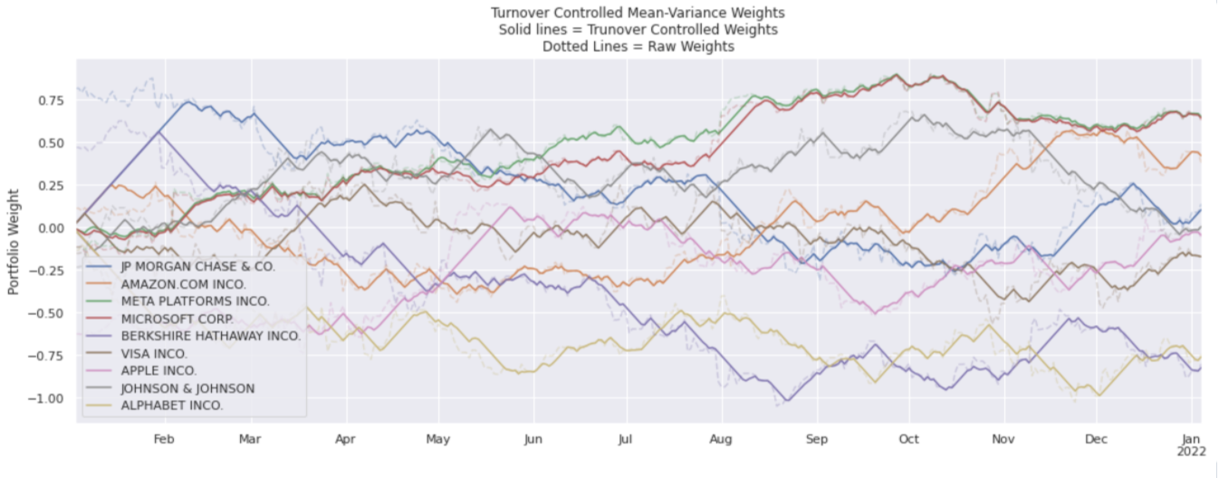
Turnover controlled mean-variance rolling signal

A mean-variance optimisation problem is defined, to which the turnover control requirement is added and compared:

mean_var_opt = sig.PortfolioOptimizer().require_weights_l2_penalty(value=5e-4)

mean_var_opt.require_mean_variance()

mean_var_opt.require_long_short_neutral()

Turnover control requires starting from pervious weights. A function is defined to apply the optimisation using the previous optimised weights on a rolling basis.

If a max_weight_change is passed, the function will apply the turnover optimisation:

def optimised_weights_over_lookback(lookback=365, max_weight_change = None):
    
    turnover_lookback = pd.DateOffset(days=lookback)
    
    weights_by_date = {}
        
    lookback_eval_dates = pd.date_range(START_DATE + turnover_lookback, env.asofdate)
    
    for lookback_end in tqdm(lookback_eval_dates):
        
        lookback_start = lookback_end - turnover_lookback

        lookback_returns_df = single_stock_returns_df.loc[lookback_start:lookback_end]

        if lookback_returns_df.index[-1] == lookback_end:
            lookback_returns_df = lookback_returns_df.iloc[:-1]
        
        opt = mean_var_opt.copy()
        
        if max_weight_change:
            
            if weights_by_date:
                previous_weights = list(weights_by_date.values())[-1]
            else:
                previous_weights = pd.Series({c:0 for c in company_names})
            
            opt = opt.require_limited_weights_turnover(
                initial_weights=previous_weights,
                max_weight_change=max_weight_change
            )
            
        weights_by_date[lookback_end] = opt.calculate_weights(lookback_returns_df)
        
    return pd.DataFrame(weights_by_date).T.sort_index()

mean_var_signal_df = optimised_weights_over_lookback()
mean_var_to_signal_df = optimised_weights_over_lookback(max_weight_change = 0.02)

Two sets of weights have been calculated on a rolling basis:

• Mean variance

• Turnover optimised mean variance

The two weights data frames are compared in the following plots. The turnover controlled version of the signal limits the daily trading but still closely matches the raw signal. The solid lines show the turnover controlled weights in comparison to the dotted lines of the raw signal.

colors=[f'C{i}' for i in range(len(company_names))]
mean_var_to_signal_df.plot(color=colors)
mean_var_signal_df.plot(ax = plt.gca(), color=colors, alpha=0.3, legend=False, ls='--')
plt.gca().set(ylabel='Portfolio Weight', title='Turnover Controlled Mean-Variance Weights\nSolid lines = Trunover Controlled Weights\nDotted Lines = Raw Weights');

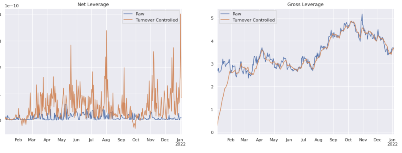
Within numerical accuracy, the net leverage of the optimiser is held to zero, as there is a long-short neutral requirement. The gross leverage is allowed to fluctuate but the turnover controlled version takes some time to build up from zero.

fig, (ax1, ax2) = plt.subplots(1, 2)

mean_var_signal_df.sum(axis=1).plot(label='Raw', ax=ax1)
mean_var_to_signal_df.sum(axis=1).plot(label='Turnover Controlled', ax=ax1)
ax1.set_title('Net Leverage')

mean_var_signal_df.abs().sum(axis=1).plot(label='Raw', ax=ax2)
mean_var_to_signal_df.abs().sum(axis=1).plot(label='Turnover Controlled', ax=ax2)
ax2.set_title('Gross Leverage')

[a.legend() for a in (ax1, ax2)];

Benchmark tracking

An equally weighted benchmark is defined:

PROBLEM_WEIGHTS['Benchmark'] = pd.Series(
    index= company_names,
    data = [1 / len(company_names)] * len(company_names)
)

run_optimisation_on_basket('Benchmark')

The require_tracking_error_upper_bound method allows optimisation of a portfolio within a tracking error, applied via the ann_te_pct variable as 10%:

tracking_error_opt = sig.PortfolioOptimizer().require_tracking_error_upper_bound(
    benchmark_weights=PROBLEM_WEIGHTS['Benchmark'],
    ann_te_pct=10
)

tracking_error_opt.require_minimum_variance()

tracking_error_opt.require_fully_invested()

PROBLEM_WEIGHTS['Tracking Error'] = tracking_error_opt.calculate_weights(single_stock_returns_df)

run_optimisation_on_basket('Tracking Error')

ax1, ax2 = plot_optimisation_results('Tracking Error')

STRATEGIES['Benchmark'].history().plot(ax=ax2, color='C2', label='Benchmark')

ax2.legend();

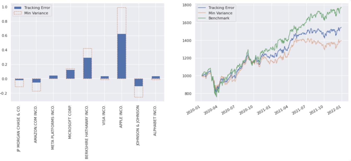
The following code validates the optimiser, solved for a tracking error of 10%:

Input

strat_returns = STRATEGIES['Tracking Error'].history().pct_change()

benchmark_returns = STRATEGIES['Benchmark'].history().pct_change()

delta_returns = strat_returns.sub( benchmark_returns, fill_value=0)
    
print(f"Realised Tracking Error with benchmark: {np.sqrt(252) * delta_returns.std():.2%}")

Output

Realised Tracking Error with benchmark: 9.93%

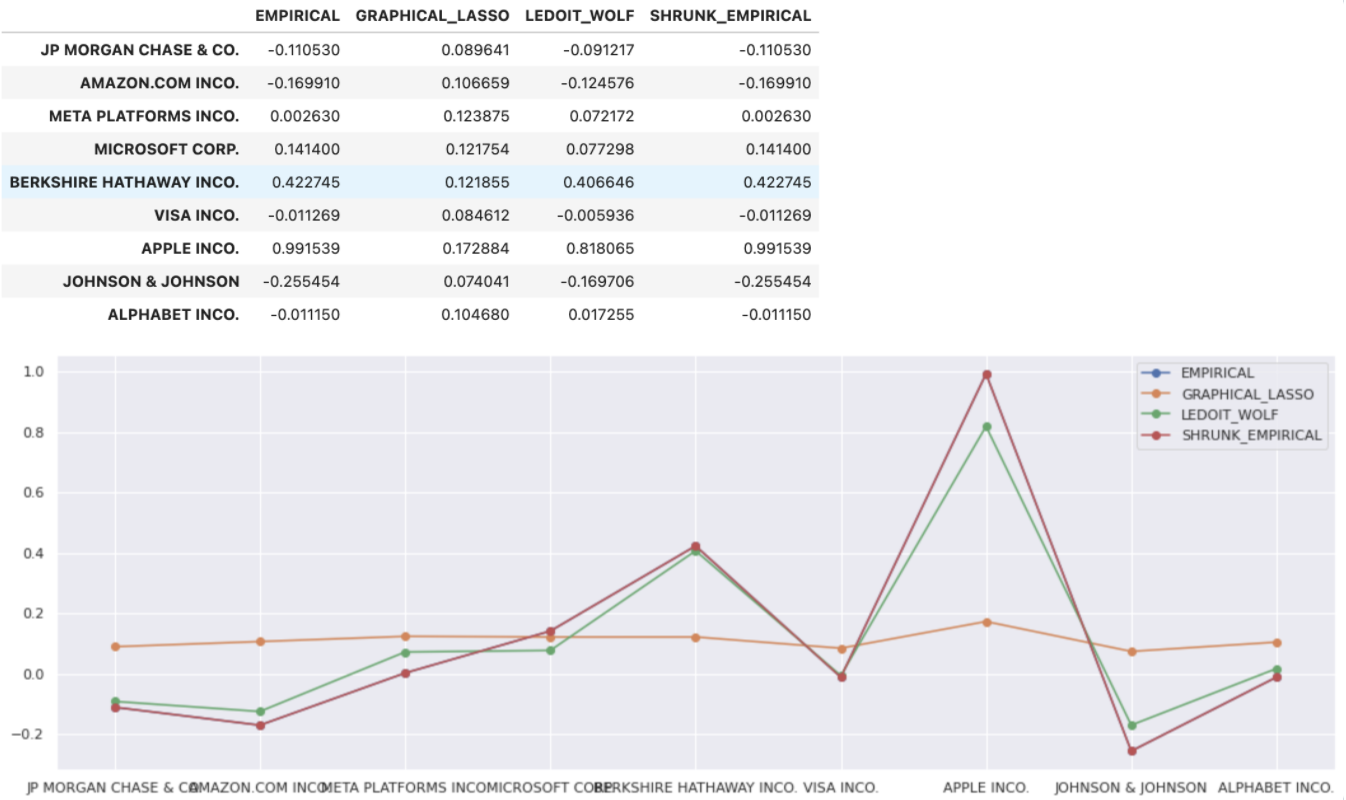
Shrinking covariance matrix

Different covariance_estimation_methods can be applied to our PortfolioOptimizer to yield different solutions. Minimum variance is used in the following example:

COV_TYPE_WEIGHTS = {}

for cov_type in ['EMPIRICAL', 'GRAPHICAL_LASSO', 'LEDOIT_WOLF', 'SHRUNK_EMPIRICAL']:
    
    cov_opt = sig.PortfolioOptimizer(
        fo_kwargs={'factor_exposure_kwargs':{'covariance_estimation_method': cov_type}}
    )
    
    cov_opt.require_minimum_variance()
    
    cov_opt.require_fully_invested()
    
    COV_TYPE_WEIGHTS[cov_type] = cov_opt.calculate_weights(single_stock_returns_df)

cov_df = pd.DataFrame(COV_TYPE_WEIGHTS)
cov_df.plot(marker='o')
cov_df

Rolling optimisations

PortfolioOptimizer objects can be passed into the allocation function of the SignalStrategy or EquityFactorBasket to be applied on a rolling basis:

po = (sig.PortfolioOptimizer().require_minimum_variance().require_fully_invested())

ss = sig.SignalStrategy(
    currency='USD',
    start_date=start_date,
    rebalance_frequency='1BD',
    signal_name=signal.name,
    allocation_function=sig.signal_library.allocation.optimized_allocations,
    allocation_kwargs={**po.signal_strategy_allocation_kwargs()}
)