Simulations & scenarios

This page shows how simulation adapters can be added for a simple momentum strategy.
SigTech platform's flexible data adapter system allows data to be replaced with artificial data. This is useful for scenario analysis, running simulations and checking strategies for possible overfitting.
Learn more: Example notebooks​
Environment
This section will import relevant internal and external libraries, as well as setting up the platform environment. 
Learn more: Environment setup​
1
import sigtech.framework as sig
2
from sigtech.framework.infra.data_adapter.simulations.simulation_adapter import SimAdapter
3
from sigtech.framework.infra.objects.dtypes import StringType, IntType, DictType
4
from sigtech.framework.schedules import SchedulePeriodic
5
from sigtech.framework.schedules.strategy import StrategySchedule
6
​
7
import datetime as dtm
8
import pandas as pd
9
import numpy as np
10
import seaborn as sns
11
​
12
sns.set(rc={'figure.figsize': (18, 6)})
13
​
14
if not sig.config.is_initialised():
15
    env = sig.config.init()
Copied!
Dates to be used when running analysis and scenarios:
1
past_date = dtm.datetime(2019, 1, 4, 11, 0)
2
future_date = dtm.datetime(2021, 10, 1, 11, 0)
Copied!
The original data & tradable instrument
Construct a simple momentum signal of the Eurostoxx index and create a tradable version of the index to trade using the signal. The index is plotted in the following example.
Use obj.get, a generic object retrieving API that can be used on any platform object, such as individual instruments or strategies. This goes to a database, an object cache or builds the object on the fly.
1
index_ts = sig.obj.get('SX5E INDEX').history()
2
instr_sx5e = sig.TradableIndex(underlying='SX5E INDEX', currency='EUR')
3
instr_sx5e.history().loc[:past_date].plot();
Copied!
A signal is defined in the example below by providing a new signal function, which retrieves the index data and evaluates the average return for the last 21 periods. The negative sign of this average is then used for a mean-reversion signal.
Defining a simple mean-reversion strategy
1
def signal_fn():
2
    mean_reversion_signal = - \
3
        np.sign(sig.obj.get('SX5E INDEX').history(
4
        ).pct_change().rolling(window=21).mean())
5
    return mean_reversion_signal.dropna().to_frame('SX5E')
6
​
7
​
8
signal_obj = sig.Signal(function=lambda: signal_fn())
Copied!
In the following example the building block SignalStrategy is used to turn a time series of signals into a tradable strategy which can be backtested. 
Learn more: Signal Strategy​
1
start_date = dtm.date(2010, 1, 4)
2
example_strategy_1 = sig.SignalStrategy(
3
    start_date=start_date,
4
    end_date=past_date,
5
    currency='EUR',
6
    signal_name=signal_obj.name,
7
    rebalance_frequency='EOM',
8
    allocation_function=sig.signal_library.allocation.identity,
9
    instrument_mapping={'SX5E': instr_sx5e.name},
10
    convert_long_short_weight=False,
11
)
Copied!
Python
Output
1
example_strategy_1.history().plot()
Copied!
Modifying the data using a simulation adapter
As the historic performance has been obtained, the performance that would be achieved if the data were modified is important. This can be achieved by introducing a simulation adapter, which can be dynamically added or removed from the data service. It obtained the raw data from the underlying data adapters and feed a modified version to the user. This allows various modifications to be performed.
A few examples include:
Moving a window of original data to a new time to be replayed. The replay can either be in absolute, difference or return space.
Perturbing the original data.
Substituting the original data with randomly generated data.
In the following example we obtain a simulation adapter, push it on to the data service and add a modifier. In this case the modifier acts on the Eurostoxx index data by shifted the original level by a normally distributed random quantity.
1
sim_adapter = SimAdapter()
2
sim_adapter.push_to_data_service()
3
​
4
sim_adapter.add_normal_timeseries_modifier(
5
    'SX5E INDEX',
6
    original_weight=1.0,
7
    change_type='PRICE',
8
    mean_override=0.0,
9
    std_override=10.0
10
)
Copied!
The caches in the platform need clearing to allow the new data to flow through:
1
sig.config.configured_env().object.clear_object_data()
Copied!
Now the modifier has been added we can retrieve the data and see a perturbation compared to the original level.
1
(sig.obj.get('SX5E INDEX').history() - index_ts).loc[:past_date].plot();
Copied!
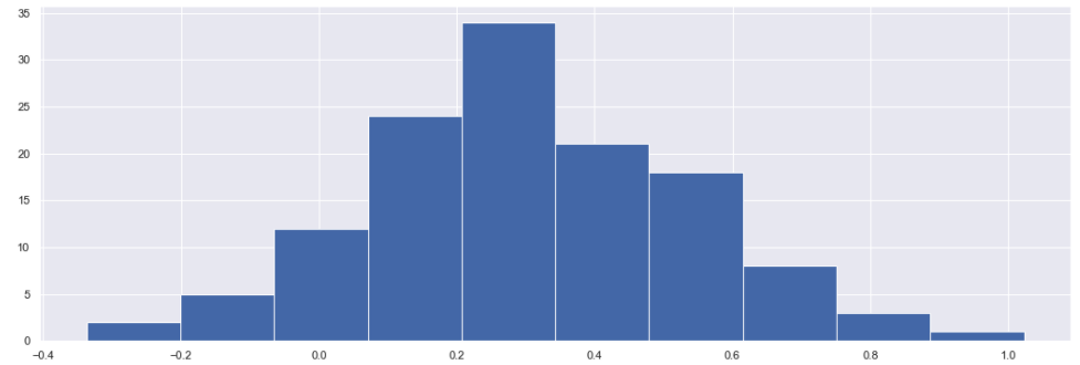
The strategy can be run multiple times using different perturbations, which are defined by a seed on the simulation adapter. The returns are all plotted below for 128 runs and the total return each time is recorded.
1
returns = []
2
for s in range(128):
3
    sim_adapter.clear_simulation()
4
    sig.config.configured_env().object.clear_object_data()
5
    sim_adapter.seed = s
6
    total_return = example_strategy_1.history().dropna()
7
    returns.append((total_return.iloc[-1] / total_return.iloc[0]) - 1)
8
    np.log(total_return).plot(color='r', alpha=0.01)
Copied!
The distribution of returns:
1
pd.Series(returns).hist(bins=10);
Copied!
As the current simulation adapter is no longer needed, remove it from the data service and clear the caches:
1
sim_adapter.remove_from_data_service()
2
sig.config.configured_env().object.clear_object_data()
3
sig.config.configured_env().fx_cross.clear_cache()
Copied!
Future scenarios
In the following example an FX hedged version of the previous strategy is run in to the future.
The FX Forward Hedging Strategy
The previous strategy is based in EUR. We can wrap it in by using the FXForwardHedgingStrategy to hedge the FX risk for a USD version.
1
hedged_instr_nky = sig.FXForwardHedgingStrategy(
2
    start_date=start_date,
3
    end_date=past_date,
4
    strategy_name=example_strategy_1.name,
5
    currency='USD',
6
    hedging_tenor='1M',
7
    exposure_rebalance_threshold=0.02,
8
    hedge_rebalance_threshold=0.02,
9
    use_holdings_for_hedge_ccy = True,
10
)
Copied!
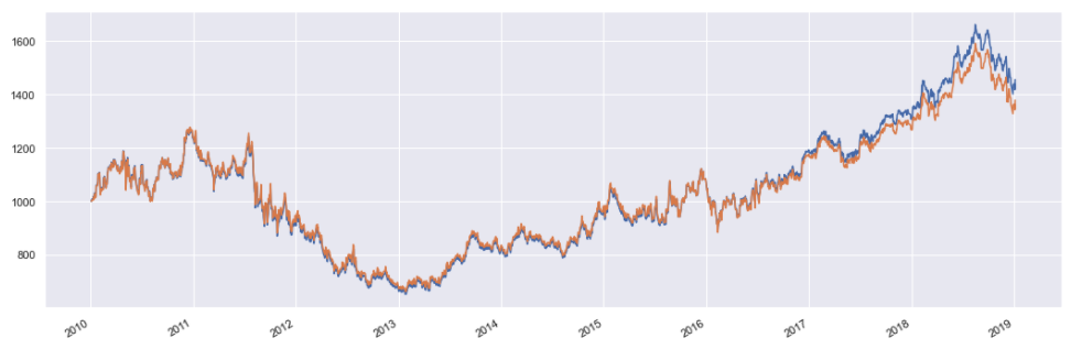
The performance of the hedged version is shown against the unhedged version:
1
hedged_instr_nky.history().plot()
2
example_strategy_1.history().plot();
Copied!
Adding a simulation adapter to replay history
Create a simulation adapter and push it to the data service. In this example, add modifiers to move data from the past in to the future. As forward is now being included in the strategy, move the curves:
1
future_sim_adapter = SimAdapter()
2
future_sim_adapter.push_to_data_service()
3
​
4
replay_start = dtm.date(2010, 1, 1)
5
​
6
future_sim_adapter.add_move_timeseries_modifier('SX5E INDEX',
7
                                                change_type='RETURN',
8
                                                original_start=replay_start,
9
                                                fill_start=past_date.date())
10
future_sim_adapter.add_move_timeseries_modifier('EURUSD CURNCY',
11
                                                change_type='RETURN',
12
                                                original_start=replay_start,
13
                                                fill_start=past_date.date())
14
future_sim_adapter.add_move_curve_modifier('USD.D CURVE',
15
                                           original_start=replay_start,
16
                                           fill_start=past_date.date())
17
future_sim_adapter.add_move_curve_modifier('USD.FX CURVE',
18
                                           original_start=replay_start,
19
                                           fill_start=past_date.date())
20
future_sim_adapter.add_move_curve_modifier('EUR.FX CURVE',
21
                                           original_start=replay_start,
22
                                           fill_start=past_date.date())
23
​
24
sig.config.configured_env().object.clear_object_data()
Copied!
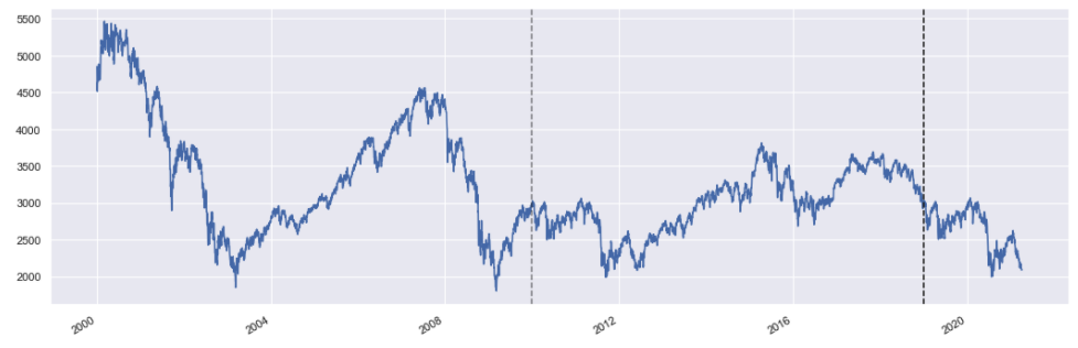
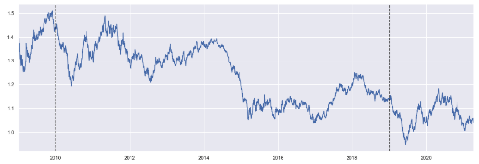
The retrieved data now shows the returns being replayed in to the future:
1
ax = sig.obj.get('SX5E INDEX').history().plot()
2
ax.axvline(past_date, color='k', linestyle='--')
3
ax.axvline(replay_start, color='k', linestyle='--', alpha=0.5);
Copied!
1
ax = sig.obj.get('EURUSD CURNCY').history().plot()
2
ax.axvline(past_date, color='k', linestyle='--')
3
ax.axvline(replay_start, color='k', linestyle='--', alpha=0.5);
Copied!
The strategies can be redefined to run up to this future date. The performance is then calculated:
1
start_date = dtm.date(2010, 1, 4)
2
future_example_strategy = sig.SignalStrategy(
3
    start_date=start_date,
4
    end_date=future_date,
5
    currency='EUR',
6
    signal_name=signal_obj.name,
7
    rebalance_frequency='EOM',
8
    allocation_function=sig.signal_library.allocation.identity,
9
    instrument_mapping={'SX5E': instr_sx5e.name},
10
    convert_long_short_weight=False,
11
)
12
​
13
hedged_instr = sig.FXForwardHedgingStrategy(
14
    start_date=start_date,
15
    end_date=future_date,
16
    strategy_name=future_example_strategy.name,
17
    currency='USD',
18
    hedging_tenor='1M',
19
    exposure_rebalance_threshold=0.02,
20
    hedge_rebalance_threshold=0.02,
21
)
22
​
23
ax = hedged_instr.history().plot(color='r')
24
future_example_strategy.history().plot(ax=ax, color='b')
25
ax.axvline(past_date, color='k', linestyle='--');
Copied!
FX Barrier Hedging Strategy
We can also hedge using FX Barrier options. The following example defines a strategy to do this:
1
class FXBarrierHedgingStrategy(sig.DailyStrategy):
2
    # Input Checking
3
    strategy_name = StringType(required=True)
4
    maturity = StringType(required=True)
5
    rebalance_frequency = StringType(required=True)
6
    group_name = StringType(required=True)
7
    bdc = StringType(default=sig.calendar.BDC_PRECEDING)
8
​
9
    def __init__(self):
10
        super(FXBarrierHedgingStrategy, self).__init__()
11
        self.option_group = sig.obj.get(self.group_name)
12
        self._strategy = sig.obj.get(self.strategy_name)
13
        self.over = self._strategy.currency
14
        self.under = self.currency
15
​
16
    def schedule_information(self):
17
        """ set the holiday calendar for rebalancing - Here we use the the same holidays as the global trading manager """
18
        return StrategySchedule(holidays=sig.TradingManager.instance().trading_holidays)
19
​
20
    def get_rebalance_dates(self):
21
        """
22
        helper function to get all the rebalance dates based on the rebalance schedule and market holidays
23
        """
24
        first_date = self.calendar_schedule().next_data_date(self.start_date)
25
        all_dates = sig.SchedulePeriodic(self.start_date, self.calculation_end_date(),
26
                                     self.history_schedule().approximate_holidays(),
27
                                     frequency=self.rebalance_frequency, bdc=self.bdc).all_data_dates()[1:]
28
        return [first_date] + all_dates
29
​
30
    def strategy_initialization(self, dt):
31
        """ This is the first function to start the strategy building process. """
32
        self.add_method(self.first_entry_date, self.push_strategy)
33
​
34
        rebalance_dates = self.get_rebalance_dates()
35
​
36
        for d in rebalance_dates:
37
            self.add_method(d, self.enter_barrier_option_positions)
38
​
39
    def push_strategy(self, dt):
40
​
41
        self.add_position_target(dt, self.strategy_name, 1.0, unit_type='WEIGHT')
42
        self.add_method(self.valuation_dt(dt.date()),
43
                           self.clean_up_foreign_cash)
44
​
45
    def clean_up_foreign_cash(self, dt):
46
        for cash_instrument, quantity in self.positions.iterate_cash_positions(dt):
47
            if cash_instrument.currency != self.currency:
48
                self.add_fx_spot_trade(dt, self.currency,
49
                                       cash_instrument.currency, -quantity)
50
​
51
    def enter_barrier_option_positions(self, dt):
52
        """ This process determines the barrier option parameters. """
53
​
54
        # first close out existing fx forwards
55
        for instrument, quantity in self.positions.iterate_instruments(dt):
56
            if instrument.is_option():
57
                self.add_position_target(dt, instrument.name, 0.0, unit_type='WEIGHT')
58
​
59
        size_date = self.size_date_from_decision_dt(dt)
60
        notional_ccy = self.valuation_price(size_date, ccy=self.over)
61
​
62
        maturity_date = self.option_group.convert_maturity_tenor_to_date(
63
            size_date, self.maturity, target_maturity_weekday=3)
64
​
65
        # Use the spot price
66
        atm = sig.obj.get(self.option_group.underlying).history().asof(pd.to_datetime(size_date))
67
​
68
        barrier_option = self.option_group.get_option(
69
            'Put', atm, size_date, maturity_date, barrier_type='KI', barrier=atm * 0.99)
70
​
71
        self.add_position_target(dt, barrier_option.name, notional_ccy)
Copied!
1
ki_hedged_instr = FXBarrierHedgingStrategy(
2
    currency='USD',
3
    strategy_name=future_example_strategy.name,
4
    start_date=start_date,
5
    end_date=past_date,
6
    group_name='EURUSD OTC OPTION GROUP',
7
    maturity='3M',
8
    rebalance_frequency='3M',
9
)
10
​
11
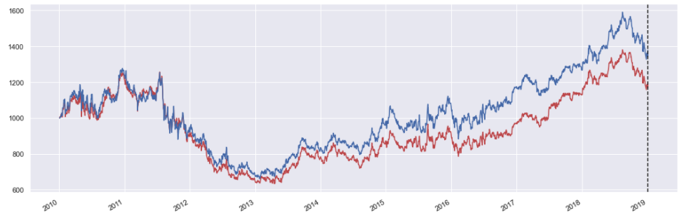
ax = ki_hedged_instr.history().plot(color='r')
12
example_strategy_1.history().plot(ax=ax, color='b')
13
ax.axvline(past_date, color='k', linestyle='--');
Copied!
​
Input
Output
1
ki_hedged_instr.timeline_holdings.display(
2
    full=True,
3
    start_dt=ki_hedged_instr.valuation_dt(start_date),
4
    end_dt=ki_hedged_instr.valuation_dt(dtm.date(2010, 5, 1))
5
)
Copied!
1
----------2010-01-05 07:30:00+00:00----------
2
          +692.6167 Units Buy outright EURUSD 20100331 PUT 1.4437999999999995 KI1.4293619999999996 7F4FF7C2 CURNCY 2010-01-05T16:00:00+00:00
3
            +0.6939       EUR ED8BED6C SS STRATEGY
4
          -693.8728       EUR CASH
5
        +1,000.0014       USD CASH
6
----------2010-01-05 16:00:00+00:00----------
7
          +692.6167       EURUSD 20100331 PUT 1.4437999999999995 KI1.4293619999999996 7F4FF7C2 CURNCY
8
            +0.6939       EUR ED8BED6C SS STRATEGY
9
          -693.8728       EUR CASH
10
          +977.1270       USD CASH
11
----------2010-01-05 23:59:59+00:00----------
12
          +692.6167       EURUSD 20100331 PUT 1.4437999999999995 KI1.4293619999999996 7F4FF7C2 CURNCY
13
            +0.6939       EUR ED8BED6C SS STRATEGY
14
           -19.6863       USD CASH
15
----------2010-01-29 16:00:00+00:00----------
16
          +692.6167       EURUSD 20100331 PUT 1.4437999999999995 KI1.4293619999999996 7F4FF7C2 CURNCY
17
            +0.6939       EUR ED8BED6C SS STRATEGY
18
           -19.6878       USD CASH
19
----------2010-02-26 16:00:00+00:00----------
20
          +692.6167       EURUSD 20100331 PUT 1.4437999999999995 KI1.4293619999999996 7F4FF7C2 CURNCY
21
            +0.6939       EUR ED8BED6C SS STRATEGY
22
           -19.6897       USD CASH
23
----------2010-03-31 15:00:00+00:00----------
24
            +0.6939       EUR ED8BED6C SS STRATEGY
25
           +43.0931       USD CASH
26
----------2010-03-31 16:00:00+00:00----------
27
            +0.6939       EUR ED8BED6C SS STRATEGY
28
           +43.0931       USD CASH
29
----------2010-04-01 06:30:00+00:00----------
30
          +820.6550 Units Buy outright EURUSD 20100702 PUT 1.3531499999999994 KI1.3396184999999994 0BCCAF85 CURNCY 2010-04-01T15:00:00+00:00
31
            +0.6939       EUR ED8BED6C SS STRATEGY
32
           +43.0933       USD CASH
33
----------2010-04-01 15:00:00+00:00----------
34
          +820.6550       EURUSD 20100702 PUT 1.3531499999999994 KI1.3396184999999994 0BCCAF85 CURNCY
35
            +0.6939       EUR ED8BED6C SS STRATEGY
36
           +18.9453       USD CASH
37
----------2010-04-30 16:00:00+00:00----------
38
          +820.6550       EURUSD 20100702 PUT 1.3531499999999994 KI1.3396184999999994 0BCCAF85 CURNCY
39
            +0.6939       EUR ED8BED6C SS STRATEGY
40
           +18.9482       USD CASH
Copied!