Position rounding

This page shows the platform’s functionality to investigate the impact of rounding off orders on the strategy performance.

Orders have a minimum size and can often only be traded in discrete units. By default, the platform simulation allows fractional units, with rounding applied when trades are exported. This allows strategies to be analysed and compared without consideration for the capital allocated to them.

The platform has additional functionality to see the impact that size has, or run the simulation with the discrete sizes enforced.

Learn more: Example notebooks

Environment

This section will import relevant internal and external libraries, as well as setting up the platform environment.

Learn more: Environment setup

import sigtech.framework as sig
from sigtech.framework.instruments.bonds import GovernmentBond

import datetime as dtm
import pandas as pd
import pytz
import seaborn as sns

sns.set(rc={'figure.figsize': (18, 6)})

if not sig.config.is_initialised():
    sig.config.init()
    sig.config.set(sig.config.FORCE_ORDER_ROUNDING, True)

Unit rounding definitions

The tradable sizes for each instrument vary and are defined on the instrument classes.

An example for government bonds:

Input:

GovernmentBond.rounded_units??

Output:

Signature: GovernmentBond.rounded_units(self, units, dt, to_trade=True)
Source:
    def rounded_units(self, units, dt, to_trade=True):
        """Round bond face values to multiples of 1000"""
        return self.positions_to_units(int(self.units_to_positions(units, dt) / 1000), dt) * 1000
File:      ~/code/framework/sigtech/framework/instruments/bonds.py
Type:      function
If required these settings can be adjusted. An example for adjusting this is given in the code below.

from sigtech.framework.instruments.bonds import GovernmentBond

def rounded_units(self, units, dt, to_trade=True):
    """Round bond face values to multiples of 10000"""
    return self.positions_to_units(int(self.units_to_positions(units, dt) / 10000), dt) * 10000

GovernmentBond.rounded_units = rounded_units

Large AUM strategy example

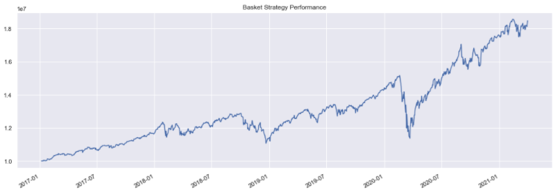
To observe the impact of this flag we can create a simple basket of two rolling future strategies. Each of the rolling futures strategies are initialised with an AUM of 1m USD and the basket has 10m USD:

def get_rfs(contract_code: str) -> sig.RollingFutureStrategy:
    return sig.RollingFutureStrategy(
        currency='USD',
        start_date=dtm.date(2010, 1, 4),
        contract_code=contract_code,
        contract_sector='INDEX',
        rolling_rule='front',
        front_offset='-6:-4'
    )

ROLLING_FUTURE_START_AUM = 10 ** 6

st = sig.BasketStrategy(
    currency='USD',
    start_date=dtm.date(2017, 1, 6),
    constituent_names=[
        get_rfs('ES').clone_strategy(
            {'initial_cash': ROLLING_FUTURE_START_AUM}
        ).name,
        get_rfs('NQ').clone_strategy(
            {'initial_cash': ROLLING_FUTURE_START_AUM}
        ).name
    ],
    weights=[0.5, 0.5],
    rebalance_frequency='EOM',
    initial_cash=10000000,
)

Input:

st.history().plot(title='Basket Strategy Performance');

Output:

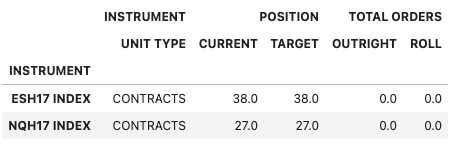
All the trades are in whole units:

Input:

st.inspect.evaluate_trades(dtm.datetime(2017, 1, 10, tzinfo=pytz.utc))

Output:

Small AUM strategy example

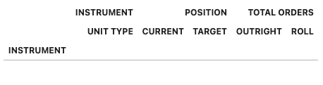
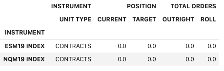
If the size of the basket is reduced to 100,000 USD, it is now too small to support the holdings of the rolling future strategies and no positions are held:

st2 = sig.BasketStrategy(
    currency='USD',
    start_date=dtm.date(2017, 1, 6),
    constituent_names=[
        get_rfs('ES').clone_strategy(
            {'initial_cash': ROLLING_FUTURE_START_AUM}
        ).name,
        get_rfs('NQ').clone_strategy(
            {'initial_cash': ROLLING_FUTURE_START_AUM}
        ).name
    ],
    weights=[0.5, 0.5],
    rebalance_frequency='EOM',
    initial_cash=100000,
)

Input:

st2.inspect.evaluate_trades(dtm.datetime(2017, 1, 10, tzinfo=pytz.utc))

Output:

Rounding impact summary

In addition to the flag provided in the configuration, each strategy has a method to investigate the impact of trading it with different allocations.

Note: this is independent of the FORCE_ORDER_ROUNDING flag, so does not require it to be active.

Call the approximate_rounding_summary method on the strategy to generate a report:

Input:

impact_data = st.analytics.approximate_rounding_summary(steps=24)
impact_data.plot(subplots=True);

Output:

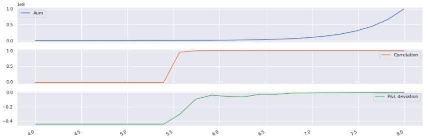
The performance of this basket drops off near an AUM of 10e5.5 USD:

Input:

st.inspect.evaluate_trades(dtm.datetime(2019, 4, 10, tzinfo=pytz.utc), aum=10**5.5)

Output:

Impact approximation

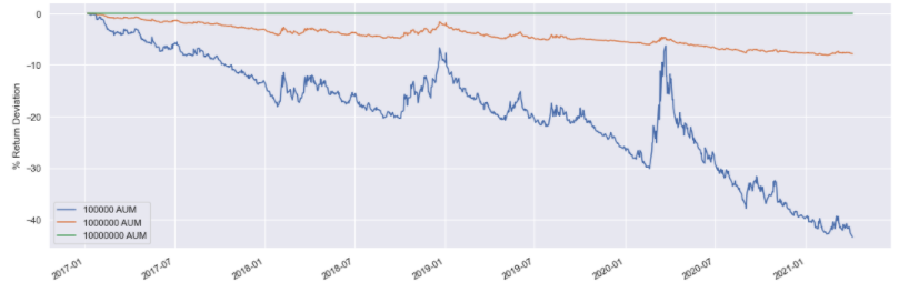
The deviation from the simulated performance can also be observed over the history using the approximate_rounding_impact method on the strategy.

Input:

ax = (100 * pd.concat(
    [st.analytics.approximate_rounding_impact(initial_aum=10 ** x).rename(str(10 ** x) + ' AUM') for x in (5, 6, 7)],
    axis=1)).plot()
ax.set_ylabel('% Return Deviation');

Output: